Semantic Search and Information Retrieval with Transformers -- RAG Fundamentals
From Keywords to Neural Understanding: The Transformer Revolution in Search — Article 9
Originally published on Medium.
From Keywords to Neural Understanding: The Transformer Revolution in Search — Article 9
- The fundamental shift from lexical matching to semantic understanding
- How transformer architectures create rich, contextual embeddings that capture meaning
- Vector databases that make these embeddings searchable at scale
- Real-world applications across customer support, knowledge management, and legal discovery
- The latest advancements including RAG integration and specialized domain models
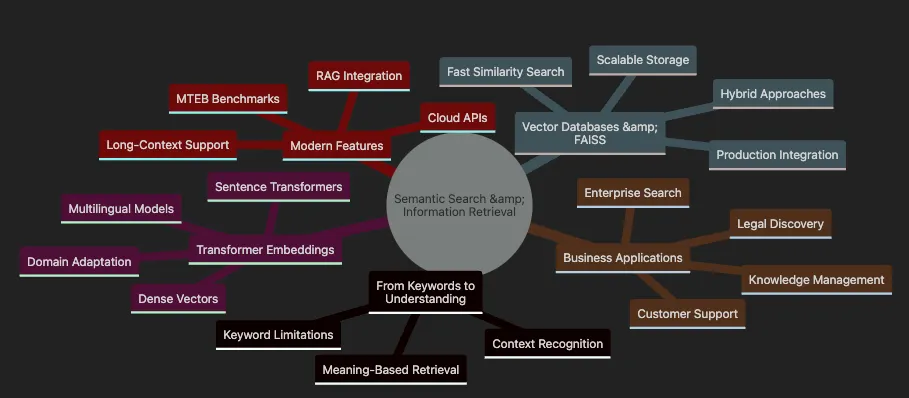
- Shows transition From Keywords to Understanding with limitations and benefits
- Covers Transformer Embeddings including models and adaptations
- Details Vector Databases & FAISS for scalable implementation
- Highlights Business Applications across industries
- Includes Modern Features like RAG and benchmarking
# Set environment variable to avoid tokenizers warning
import
 os
os.environ[
'TOKENIZERS_PARALLELISM'
] =
'false'
# Import necessary libraries
import
 numpy
as
 np
import
 pandas
as
 pd
import
 matplotlib.pyplot
as
 plt
import
 seaborn
as
 sns
from
 sentence_transformers
import
 SentenceTransformer, util
from
 rank_bm25
import
 BM25Okapi
import
 warnings
warnings.filterwarnings(
'ignore'
)
# Set up plotting style
plt.style.use(
'seaborn-v0_8-darkgrid'
)
sns.set_palette(
"husl"
)
print
(
"Libraries imported successfully!"
)
print
(
f"NumPy version:
{np.__version__}
"
)
print
(
f"Pandas version:
{pd.__version__}
"
)
- Environment Setup: Set tokenizers parallelism to avoid warnings in notebook environments
- Import Core Libraries: Load essential packages for numerical computation, data manipulation, and visualization
- Import Search Components: Load sentence transformers for semantic search and BM25 for keyword search
- Configure Visualization: Set up consistent plotting style for clear visual outputs
- Verify Installation: Print versions to ensure proper setup
import
 sys
print
(
f"Python version:
{sys.version}
"
)
# Load the sentence transformer model
print
(
"\nLoading sentence transformer model..."
)
model = SentenceTransformer(
'all-MiniLM-L6-v2'
)
print
(
"Model loaded successfully!"
)
# Test the model with a simple example
test_sentence =
"Hello, world!"
test_embedding = model.encode(test_sentence)
print
(
f"\nTest embedding shape:
{test_embedding.shape}
"
)
print
(
f"Embedding dimension:
{
len
(test_embedding)}
"
)
Python version:

3.12
.9

(main,

Apr

29

2025
,

13
:57:48)
 [
Clang

16.0
.0

(clang-1600.0.26.4)
]
Loading

sentence

transformer

model...
Model

loaded

successfully!
Test embedding shape:

(384,)
Embedding dimension:

384
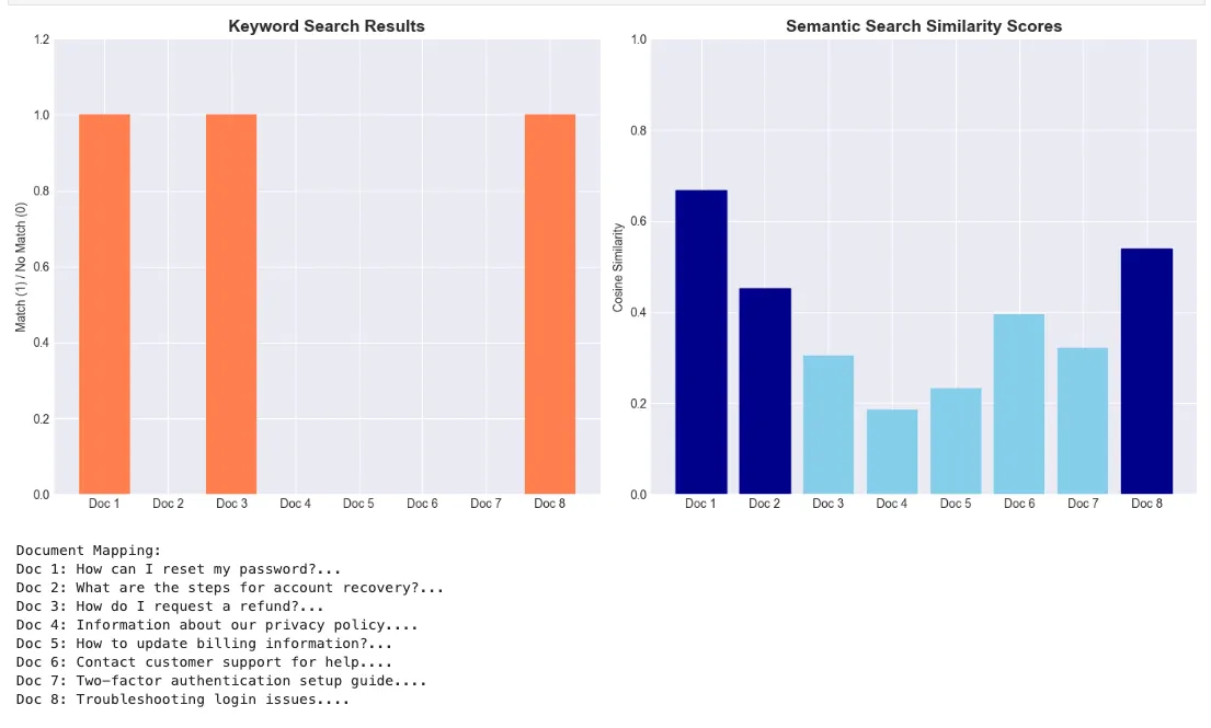
- How traditional keyword search fails when exact word matching isn’t present
- How transformer-based semantic search correctly identifies relevant content through meaning
- The practical implementation using the sentence-transformers library
- Why semantic search produces superior results for natural language queries
# Define our FAQ documents
faqs = [

"How can I reset my password?"
,

"What are the steps for account recovery?"
,

"How do I request a refund?"
,

"Information about our privacy policy."
,

"How to update billing information?"
,

"Contact customer support for help."
,

"Two-factor authentication setup guide."
,

"Troubleshooting login issues."
]
# User query that doesn't match keywords exactly
query =
"I forgot my login credentials"
print
(
f"User Query: '
{query}
'"
)
print
(
"\\\\n"
 +
"="
*
50
 +
"\\\\n"
)
Output:
User
 Query:
'I forgot my login credentials'
=
=
=
=
=
=
=
=
=
=
=
=
=
=
=
=
=
=
=
=
=
=
=
=
=
=
=
=
=
=
=
=
=
=
=
=
=
=
=
=
=
=
=
=
=
=
=
=
=
=
# Keyword Search Implementation
def

keyword_search
(
query, documents
):

"""Simple keyword matching search"""
    query_words =
set
(query.lower().split())
    matches = []


for
 doc
in
 documents:
        doc_words =
set
(doc.lower().split())

if
 query_words & doc_words:
# Intersection
            matches.append(doc)


return
 matches
# Perform keyword search
keyword_results = keyword_search(query, faqs)
print
(
"🔍 KEYWORD SEARCH RESULTS:"
)
if
 keyword_results:

for
 i, result
in

enumerate
(keyword_results,
1
):

print
(
f"
{i}
.
{result}
"
)
else
:

print
(
"  No matches found! ❌"
)

print
(
"  (No shared words between query and documents)"
)
🔍
KEYWORD

SEARCH

RESULTS
:

1
.
How

can

I

reset

my

password
?

2
.
How

do

I

request

a

refund
?

3
.
Troubleshooting

login

issues
.
- Define FAQs and Query: Create sample documents and a user question that doesn’t match keywords exactly
- Keyword Search: Split query into words, find FAQs sharing any word — misses relevant answers when wording differs
- Check Intersection: Use set intersection to find common words between query and documents
- Display Results: Show which documents matched, or indicate no matches found
- Highlight Limitation: Demonstrate how exact word matching fails for natural language queries
# Semantic Search Implementation
def

semantic_search
(
query, documents, model, top_k=
3
):

"""Semantic search using sentence transformers"""

# Encode query and documents
    query_embedding = model.encode(query, convert_to_numpy=
True
)
    doc_embeddings = model.encode(documents, convert_to_numpy=
True
)


# Calculate cosine similarities
    similarities = util.cos_sim(query_embedding, doc_embeddings)[
0
]


# Get top-k results
    top_results = similarities.argsort(descending=
True
)[:top_k]

    results = [(documents[idx],
float
(similarities[idx]))
for
 idx
in
 top_results]

return
 results
# Perform semantic search
semantic_results = semantic_search(query, faqs, model)
print
(
"\n🧠 SEMANTIC SEARCH RESULTS:"
)
for
 i, (doc, score)
in

enumerate
(semantic_results,
1
):

print
(
f"
{i}
.
{doc}
"
)

print
(
f"     (Similarity score:
{score:
.3
f}
)"
)
🧠
SEMANTIC

SEARCH

RESULTS
:

1
.
How

can

I

reset

my

password
?
     (Similarity
score
:
0.667
)

2
.
Troubleshooting

login

issues
.
     (Similarity
score
:
0.538
)

3
.
What

are

the

steps

for

account

recovery
?
     (Similarity
score
:
0.453
)
- Generate Embeddings: Convert query and documents into dense vectors capturing semantic essence
- Calculate Similarity: Use cosine similarity to measure meaning closeness between vectors
- Rank Results: Sort FAQs by similarity score — most relevant surfaces first
- Return Top Matches: Extract the most semantically similar documents
- Display with Scores: Show results with confidence scores indicating semantic similarity
- Customer Support: Users rarely phrase questions matching your documentation. Semantic search bridges this gap
- Enterprise Knowledge: Employees discover procedures using their own terminology
- Legal Compliance: Lawyers surface relevant precedents by meaning, not exact phrasing
# Create a comparison visualization
fig, (ax1, ax2) = plt.subplots(
1
,
2
, figsize=(
14
,
6
))
# Keyword search visualization
keyword_data = pd.DataFrame({

'Document'
: [
'Doc '
 +
str
(i+
1
)
for
 i
in

range
(
len
(faqs))],

'Match'
: [
1

if
 faq
in
 keyword_results
else

0

for
 faq
in
 faqs]
})
ax1.bar(keyword_data[
'Document'
], keyword_data[
'Match'
], color=
'coral'
)
ax1.set_title(
'Keyword Search Results'
, fontsize=
14
, fontweight=
'bold'
)
ax1.set_ylabel(
'Match (1) / No Match (0)'
)
ax1.set_ylim(
0
,
1.2
)
# Semantic search visualization
query_emb = model.encode(query)
doc_embs = model.encode(faqs)
all_similarities = util.cos_sim(query_emb, doc_embs)[
0
].numpy()
semantic_data = pd.DataFrame({

'Document'
: [
'Doc '
 +
str
(i+
1
)
for
 i
in

range
(
len
(faqs))],

'Similarity'
: all_similarities
})
bars = ax2.bar(semantic_data[
'Document'
], semantic_data[
'Similarity'
], color=
'skyblue'
)
ax2.set_title(
'Semantic Search Similarity Scores'
, fontsize=
14
, fontweight=
'bold'
)
ax2.set_ylabel(
'Cosine Similarity'
)
ax2.set_ylim(
0
,
1.0
)
# Highlight top 3 results
top_3_indices = all_similarities.argsort()[-
3
:][::-
1
]
for
 idx
in
 top_3_indices:
    bars[idx].set_color(
'darkblue'
)
plt.tight_layout()
plt.show()
# Print the FAQ mapping
print
(
"\nDocument Mapping:"
)
for
 i, faq
in

enumerate
(faqs):

print
(
f"Doc
{i+
1
}
:
{faq[:
50
]}
..."
)
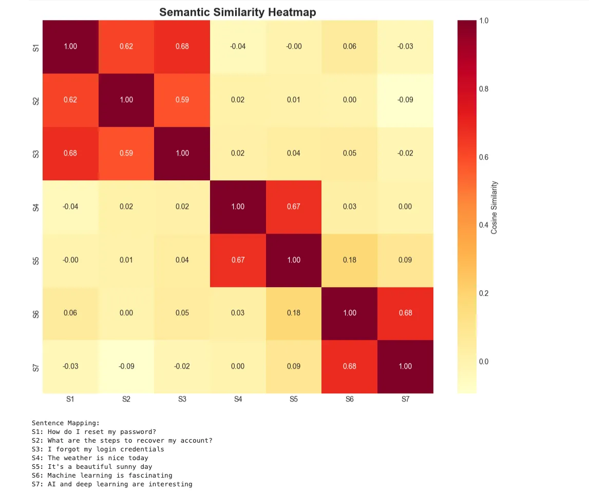
# Generate embeddings for different types of sentences
sentences = [

# Similar meanings

"How do I reset my password?"
,

"What are the steps to recover my account?"
,

"I forgot my login credentials"
,


# Different topic

"The weather is nice today"
,

"It's a beautiful sunny day"
,


# Another different topic

"Machine learning is fascinating"
,

"AI and deep learning are interesting"
]
# Generate embeddings
embeddings = model.encode(sentences)
print
(
f"Generated embeddings for
{
len
(sentences)}
 sentences"
)
print
(
f"Embedding shape:
{embeddings.shape}
"
)
Generated

embeddings

for

7

sentences
Embedding shape:

(7,

384
)
# Calculate similarity matrix
similarity_matrix = util.cos_sim(embeddings, embeddings).numpy()
# Create a heatmap visualization
plt.figure(figsize=(
10
,
8
))
sns.heatmap(similarity_matrix,
            annot=
True
,
            fmt=
".2f"
,
            cmap=
"YlOrRd"
,
            xticklabels=[
f"S
{i+
1
}
"

for
 i
in

range
(
len
(sentences))],
            yticklabels=[
f"S
{i+
1
}
"

for
 i
in

range
(
len
(sentences))],
            cbar_kws={
'label'
:
'Cosine Similarity'
})
plt.title(
"Semantic Similarity Heatmap"
, fontsize=
16
, fontweight=
'bold'
)
plt.tight_layout()
plt.show()
# Print sentence mapping
print
(
"\nSentence Mapping:"
)
for
 i, sent
in

enumerate
(sentences):

print
(
f"S
{i+
1
}
:
{sent}
"
)
from
 sklearn.manifold
import
 TSNE
# Generate more embeddings for better visualization
categories = {

"Password/Login"
: [

"How do I reset my password?"
,

"Forgot my login credentials"
,

"Account recovery steps"
,

"Can't access my account"
    ],

"Billing/Payment"
: [

"How to update payment method?"
,

"Request a refund"
,

"Billing information update"
,

"Payment failed issues"
    ],

"Technical Support"
: [

"App crashes frequently"
,

"Software bug report"
,

"Technical difficulties"
,

"System error messages"
    ]
}
# Prepare data
all_sentences = []
labels = []
colors = []
color_map = {
'Password/Login'
:
'red'
,
'Billing/Payment'
:
'green'
,
'Technical Support'
:
'blue'
}
for
 category, sents
in
 categories.items():
    all_sentences.extend(sents)
    labels.extend([category] *
len
(sents))
    colors.extend([color_map[category]] *
len
(sents))
# Generate embeddings
all_embeddings = model.encode(all_sentences)
# Apply t-SNE
tsne = TSNE(n_components=
2
, random_state=
42
, perplexity=
5
)
embeddings_2d = tsne.fit_transform(all_embeddings)
# Create visualization
plt.figure(figsize=(
10
,
8
))
for
 category
in
 categories.keys():
    mask = np.array(labels) == category
    plt.scatter(embeddings_2d[mask,
0
],
                embeddings_2d[mask,
1
],
                c=color_map[category],
                label=category,
                alpha=
0.7
,
                s=
100
)
# Add annotations
for
 i, txt
in

enumerate
(all_sentences):
    plt.annotate(
f"
{i+
1
}
"
,
                 (embeddings_2d[i,
0
], embeddings_2d[i,
1
]),
                 fontsize=
8
,
                 ha=
'center'
)
plt.xlabel(
't-SNE Component 1'
)
plt.ylabel(
't-SNE Component 2'
)
plt.title(
'Semantic Embeddings Visualization (t-SNE)'
, fontsize=
16
, fontweight=
'bold'
)
plt.legend()
plt.grid(
True
, alpha=
0.3
)
plt.tight_layout()
plt.show()
# Print sentence mapping
print
(
"\nSentence Mapping:"
)
for
 i, (sent, cat)
in

enumerate
(
zip
(all_sentences, labels)):

print
(
f"
{i+
1
}
. [
{cat}
]
{sent}
"
)
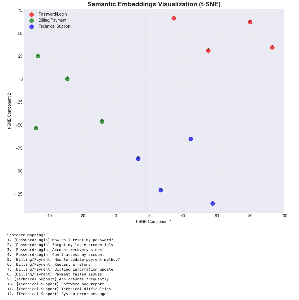
- Organize by Category: Group sentences into meaningful categories
- Prepare Labels: Track category membership for visualization
- Generate All Embeddings: Create vectors for entire dataset
- Apply Dimensionality Reduction: Use t-SNE to project to 2D space
- Visualize Clustering: Similar meanings cluster together in 2D
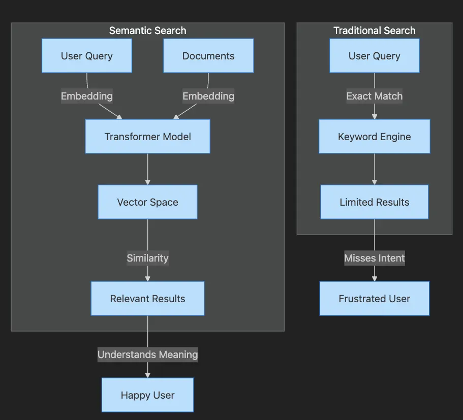
- Traditional Search path shows query going through keyword engine to limited results
- User becomes frustrated when intent is missed
- Semantic Search path shows both query and documents becoming embeddings
- Transformer creates vectors that capture meaning
- Similarity matching produces relevant results
- User achieves satisfaction through understood intent
import
 sys
print
(
f"Python version:
{sys.version}
"
)
# Load the sentence transformer model
print
(
"\\\\nLoading sentence transformer model..."
)
model = SentenceTransformer(
'all-MiniLM-L6-v2'
)
print
(
"Model loaded successfully!"
)
# Test the model with a simple example
test_sentence =
"Hello, world!"
test_embedding = model.encode(test_sentence)
print
(
f"\\\\nTest embedding shape:
{test_embedding.shape}
"
)
print
(
f"Embedding dimension:
{
len
(test_embedding)}
"
)
- Verify Python Version: Ensure we’re using Python 3.12.9 for consistency
- Load Transformer: Initialize model that creates semantic embeddings
- Test Embedding: Generate a sample embedding to verify model is working
- Check Dimensions: Confirm embeddings are 384-dimensional vectors
- Ready for Search: Model is prepared to encode documents and queries
# Import our hybrid search implementation
import
 sys
sys.path.append(
'../src'
)
from
 hybrid_search
import
 HybridSearchEngine
# Create sample documents
documents = [

"How to reset your password: Click forgot password on login page"
,

"Account recovery steps for forgotten credentials"
,

"Password reset instructions and security guidelines"
,

"Update your profile information in account settings"
,

"Two-factor authentication setup guide"
,

"Troubleshooting login issues and access problems"
,

"Security best practices for strong passwords"
,

"How to change your email address in settings"
,

"Recovering locked accounts after failed login attempts"
,

"Password manager recommendations for secure storage"
]
# Initialize hybrid search engine
hybrid_engine = HybridSearchEngine()
hybrid_engine.index_documents(documents)
print
(
"Hybrid search engine initialized!"
)
Initializing

hybrid

search

engine...
Semantic model:

all-MiniLM-L6-v2
Weights - Keyword:

0.3
,

Semantic:

0.7
Indexing

10

documents...
Building

BM25

index...
Generating

semantic

embeddings...
Error displaying widget:

model

not

found
Indexing

completed

in

0.09

seconds
Hybrid

search

engine

initialized!
- Import Hybrid Engine: Load the hybrid search implementation that combines approaches
- Create Document Set: Prepare diverse documents covering various topics
- Initialize Engine: Create hybrid search engine with default weights
- Index Documents: Build both BM25 index and semantic embeddings
- Ready for Search: System prepared to handle queries with adaptive weighting
# Test different queries with varying lengths
test_queries = [

"reset"
,
# Very short - keyword heavy

"forgot password"
,
# Short - balanced

"I can't remember my login"
,
# Medium - balanced

"What are the steps to recover my account when I've forgotten my password?"

# Long - semantic heavy
]
# Compare search approaches
results_comparison = []
for
 query
in
 test_queries:

# Get adaptive weights
    kw_weight, sem_weight = hybrid_engine.adaptive_weighting(query)


# Perform search
    results = hybrid_engine.search(query, k=
3
, return_scores=
True
)

    results_comparison.append({

'query'
: query,

'query_length'
:
len
(query.split()),

'keyword_weight'
: kw_weight,

'semantic_weight'
: sem_weight,

'top_result'
: results[
0
][
'document'
][:
50
] +
'...'

if
 results
else

'No results'
,

'top_score'
: results[
0
][
'hybrid_score'
]
if
 results
else

0
    })
# Create comparison table
comparison_df = pd.DataFrame(results_comparison)
print
(
"\n🔍 Adaptive Weight Analysis:"
)
print
(
"="
*
80
)
display(comparison_df)
-
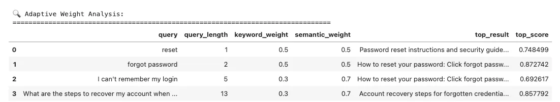
Define Test Queries: Create queries of varying lengths to test adaptive weighting
-
Calculate Weights: System automatically adjusts keyword/semantic balance based on query
-
Perform Searches: Execute hybrid search with adaptive weights
-
Collect Results: Gather top matches and scores for analysis
-
Display Analysis: Show how weights adapt to query characteristics
-
Enterprise Knowledge Bases: Employees use varied terminology. Semantic search bridges vocabulary gaps, surfacing answers regardless of phrasing.
-
Customer Support Automation: Intent-aware chatbots understand “How can I get my money back?” matches refund policies — without the word “refund.”
-
Legal and Compliance Discovery: Legal teams find relevant precedents through meaning, not just keywords — saving hours, reducing risk. This aligns with enterprise use cases I’ve covered in The Economics of Deploying Large Language Models: Costs, Value, and 99.7% Savings, and for scaling such systems, refer to my blog post Scaling Up: Debugging, Optimization, and Distributed Training — Article 17.
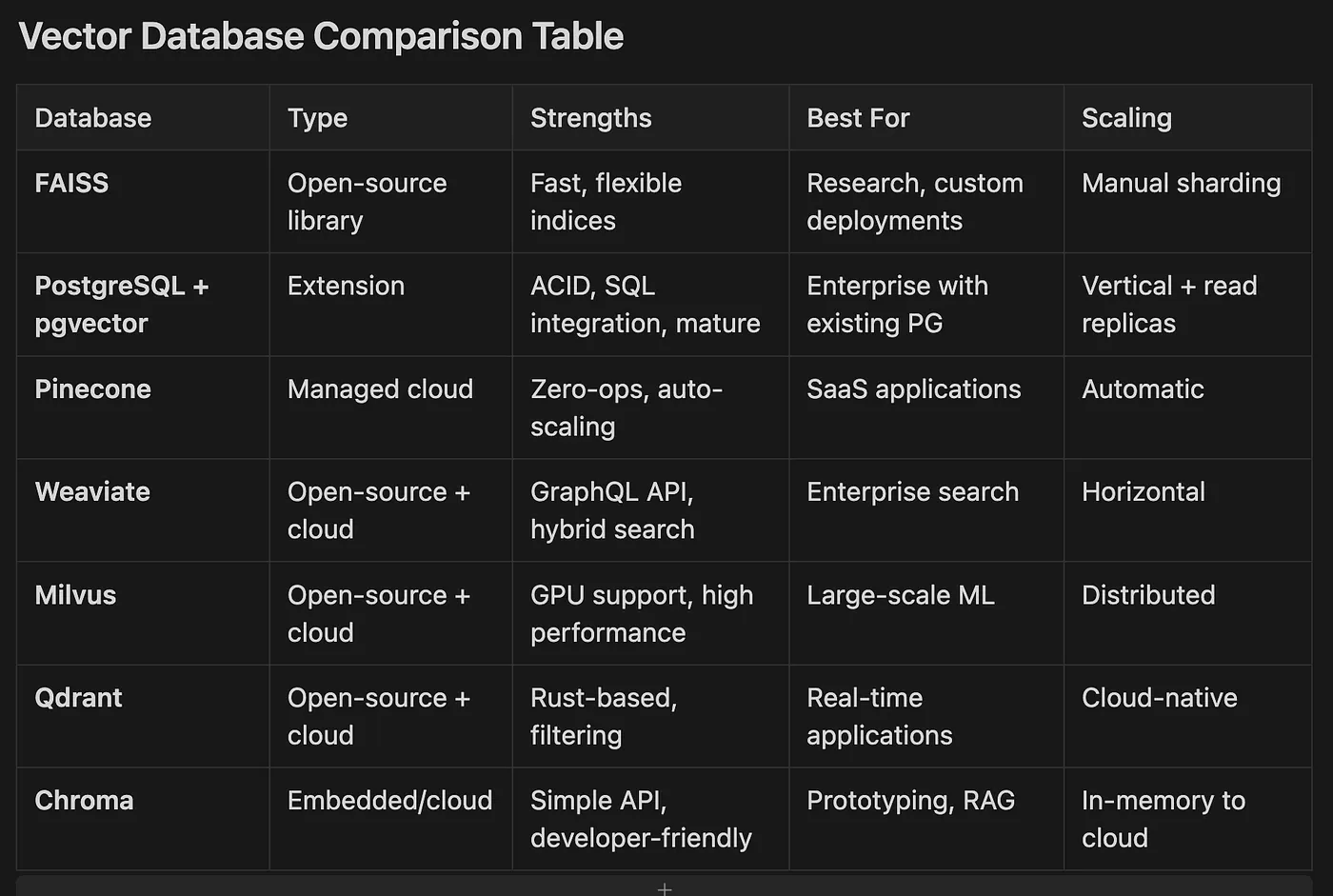
- FAISS Open-source library Fast, flexible indices Research, custom deployments Manual sharding
- PostgreSQL + pgvector Extension ACID, SQL integration, mature Enterprise with existing PG Vertical + read replicas
- Pinecone Managed cloud Zero-ops, auto-scaling SaaS applications Automatic
- Weaviate Open-source + cloud GraphQL API, hybrid search Enterprise search Horizontal
- Milvus Open-source + cloud GPU support, high performance Large-scale ML Distributed
- Qdrant Open-source + cloud Rust-based, filtering Real-time applications Cloud-native
- Chroma Embedded/cloud Simple API, developer-friendly Prototyping, RAG In-memory to cloud
- Precision: What fraction of results are relevant? High precision minimizes irrelevant noise.
- Recall: What fraction of relevant documents appeared? High recall ensures nothing important is missed.
- F1 Score: Harmonizes precision and recall into one balanced metric.
- Mean Reciprocal Rank (MRR): How high does the first relevant result appear? Top placement delights users.
- Normalized Discounted Cumulative Gain (NDCG): Evaluates entire ranking, rewarding relevant results near the top — crucial for result lists.
# Implement search quality metrics
def

calculate_metrics
(
retrieved, relevant
):

"""
    Calculate precision, recall, and F1 score
    """
    retrieved_set =
set
(retrieved)
    relevant_set =
set
(relevant)
    true_positives =
len
(retrieved_set & relevant_set)
    precision = true_positives /
len
(retrieved_set)
if
 retrieved_set
else

0
    recall = true_positives /
len
(relevant_set)
if
 relevant_set
else

0
    f1 =
2
 * (precision * recall) / (precision + recall)
if
 (precision + recall) >
0

else

0

return
 precision, recall, f1
# Example evaluation
test_cases = [
    {

'name'
:
'Perfect Match'
,

'retrieved'
: [
'doc1'
,
'doc2'
,
'doc3'
],

'relevant'
: [
'doc1'
,
'doc2'
,
'doc3'
]
    },
    {

'name'
:
'Partial Match'
,

'retrieved'
: [
'doc1'
,
'doc2'
,
'doc5'
],

'relevant'
: [
'doc2'
,
'doc3'
,
'doc5'
]
    },
    {

'name'
:
'Poor Match'
,

'retrieved'
: [
'doc1'
,
'doc4'
,
'doc6'
],

'relevant'
: [
'doc2'
,
'doc3'
,
'doc5'
]
    }
]
metrics_results = []
for

case

in
 test_cases:
    precision, recall, f1 = calculate_metrics(
case
[
'retrieved'
],
case
[
'relevant'
])
    metrics_results.append({

'Scenario'
:
case
[
'name'
],

'Precision'
: precision,

'Recall'
: recall,

'F1 Score'
: f1
    })
metrics_df = pd.DataFrame(metrics_results)
- Define Sets: Retrieved documents vs. truly relevant documents
- Calculate Intersection: Find documents that are both retrieved and relevant
- Compute Precision: Fraction of retrieved that are relevant
- Compute Recall: Fraction of relevant that were retrieved
- Calculate F1: Harmonic mean balancing precision and recall
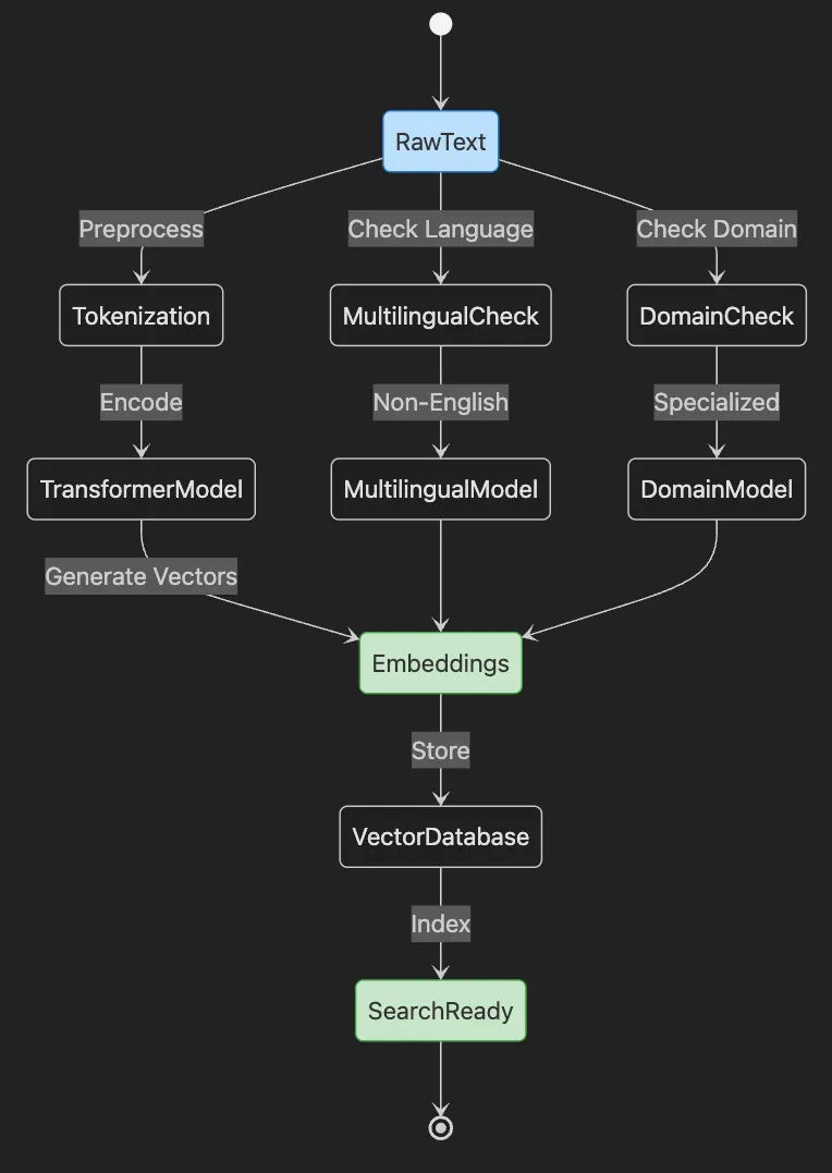
- Start with RawText that needs embedding
- Text goes through Tokenization preprocessing
- TransformerModel encodes tokens into Embeddings
- Embeddings stored in VectorDatabase and indexed
- System becomes SearchReady
- Parallel paths handle Multilingual and Domain-specific content
- What embeddings are and their importance
- Creating them with sentence transformers and modern APIs
- Storing and managing embeddings at scale
- Multilingual and domain-specific strategies
- Selecting optimal models and databases
-
“How do I reset my password?”
-
“What are the steps to recover my account?”
-
Customer question routing to relevant help articles — despite different wording
-
Support ticket clustering by issue type
-
Cross-language search focusing on meaning
-
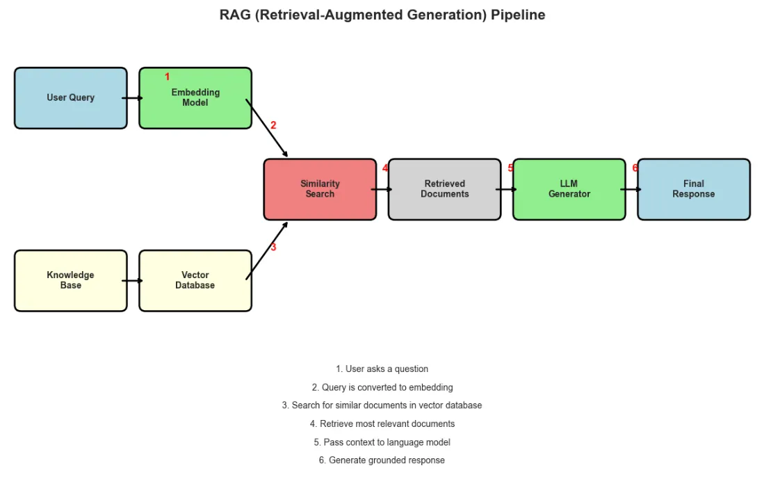
Retrieval-augmented generation (RAG) combining search with LLMs for reasoning
# Generate embeddings for different types of sentences
sentences
 = [

# Similar meanings

"How do I reset my password?"
,

"What are the steps to recover my account?"
,

"I forgot my login credentials"
,
    # Different topic
    "The weather is nice today",
    "It's a beautiful sunny day",
    # Another different topic
    "Machine learning is fascinating",
    "AI and deep learning are interesting"
]
# Generate embeddings
embeddings = model.encode(sentences)
print(f"Generated embeddings for {len(sentences)} sentences")
print(f"Embedding shape: {embeddings.shape}")
- Define Sentence Groups: Create sentences with similar and different meanings
- Generate Embeddings: Convert sentences to 384-dimensional vectors
- Verify Output: Confirm embedding dimensions match expectations
- Understand Structure: Each sentence maps to a fixed-size vector
- Ready for Comparison: Embeddings can now be compared for similarity
# Create a knowledge base
knowledge_base = [

"Our refund policy allows returns within 30 days of purchase. To initiate a refund, contact customer support with your order number."
,

"Password reset: Click 'Forgot Password' on the login page. Enter your email address and check your inbox for reset instructions."
,

"Two-factor authentication adds an extra layer of security. Enable it in your account settings under the Security tab."
,

"Premium subscription includes unlimited storage, priority support, and advanced analytics features for $19.99/month."
,

"Technical support is available 24/7 via email at [email protected] or through live chat on our website."
,

"Account suspension may occur due to policy violations. Contact support to appeal or learn more about the suspension."
,

"Data privacy: We use industry-standard encryption and never share your personal information with third parties."
,

"API rate limits: Free tier allows 1000 requests/day. Premium users get 10,000 requests/day with no throttling."
]
# Create embeddings for knowledge base
kb_embeddings = model.encode(knowledge_base)
print
(f
"Knowledge base contains {len(knowledge_base)} documents"
)
Knowledge
base
 contains
8
 documents
- Define Knowledge Base: Create documents covering various topics
- Generate KB Embeddings: Convert all documents to vectors
- Store for Retrieval: Embeddings ready for similarity search
- Enable RAG: System can now retrieve relevant context
- Support Generation: Retrieved docs provide context for answers
# Simple RAG implementation
def

simple_rag
(
query, knowledge_base, kb_embeddings, model, top_k=
2
):

"""
    Simple RAG: Retrieve relevant context and generate response
    """

# Step 1: Retrieve relevant documents
    query_embedding = model.encode(query)
    similarities = util.cos_sim(query_embedding, kb_embeddings)[
0
]
    top_indices = similarities.argsort(descending=
True
)[:top_k]


# Get retrieved documents
    retrieved_docs = [knowledge_base[idx]
for
 idx
in
 top_indices]
    retrieved_scores = [
float
(similarities[idx])
for
 idx
in
 top_indices]


# Step 2: Create context for generation
    context =
"\n\n"
.join(retrieved_docs)


# Step 3: Generate response (using a simple template for demonstration)

# In production, you would use a proper LLM here
    response =
f"""Based on the information in our knowledge base:
{context}
To answer your question about '
{query}
':
{retrieved_docs[
0
]}
This information was retrieved with
{retrieved_scores[
0
]:
.1
%}
 confidence."""


return
 response, retrieved_docs, retrieved_scores
# Test RAG system
test_questions = [

"How do I get a refund?"
,

"Is my data secure?"
,

"What are the API limits?"
]
for
 question
in
 test_questions:

print
(
f"\n
{
'='
*
60
}
"
)

print
(
f"❓ Question:
{question}
"
)
    response, docs, scores = simple_rag(question, knowledge_base, kb_embeddings, model)

print
(
f"\n📚 Retrieved Documents:"
)

for
 i, (doc, score)
in

enumerate
(
zip
(docs, scores)):

print
(
f"
{i+
1
}
. (Score:
{score:
.3
f}
)
{doc[:
80
]}
..."
)

print
(
f"\n💡 Generated Response:"
)

print
(response)
============================================================
❓ Question: How
do
 I
get
 a refund?
📚 Retrieved Documents:

1
. (Score:
0.601
) Our refund policy allows returns within
30
 days
of
 purchase.
To
 initiate a refun...

2
. (Score:
0.270
) Account suspension may occur due
to
 policy violations. Contact support
to
 appeal...
💡 Generated Response:
Based
on
 the information
in
 our knowledge base:
Our refund policy allows returns within
30
 days
of
 purchase.
To
 initiate a refund, contact customer support
with
 your
order
 number.
Account suspension may occur due
to
 policy violations. Contact support
to
 appeal
or
 learn more about the suspension.
To
 answer your question about
'How do I get a refund?':
Our refund policy allows returns within
30
 days
of
 purchase.
To
 initiate a refund, contact customer support
with
 your
order
 number.
This information was retrieved
with

60.1
% confidence.
============================================================
❓ Question:
Is
 my data secure?
📚 Retrieved Documents:

1
. (Score:
0.503
) Data privacy: We use industry-standard encryption
and
 never share your personal ...

2
. (Score:
0.306
) Two-factor authentication adds an extra layer
of
 security. Enable it
in
 your acc...
💡 Generated Response:
Based
on
 the information
in
 our knowledge base:
Data privacy: We use industry-standard encryption
and
 never share your personal information
with
 third parties.
Two-factor authentication adds an extra layer
of
 security. Enable it
in
 your account settings under the Security tab.
To
 answer your question about
'Is my data secure?':
Data privacy: We use industry-standard encryption
and
 never share your personal information
with
 third parties.
This information was retrieved
with

50.3
% confidence.
============================================================
❓ Question: What are the API limits?
📚 Retrieved Documents:

1
. (Score:
0.666
) API rate limits: Free tier allows
1000
 requests/day. Premium users
get

10
,
000
 re...

2
. (Score:
0.271
) Premium subscription includes unlimited storage, priority support,
and
 advanced ...
💡 Generated Response:
Based
on
 the information
in
 our knowledge base:
API rate limits: Free tier allows
1000
 requests/day. Premium users
get

10
,
000
 requests/day
with
 no throttling.
Premium subscription includes unlimited storage, priority support,
and
 advanced analytics features
for
 $
19.99
/month.
To
 answer your question about
'What are the API limits?':
API rate limits: Free tier allows
1000
 requests/day. Premium users
get

10
,
000
 requests/day
with
 no throttling.
This information was retrieved
with

66.6
% confidence.
- Embed Query: Convert user question to vector
- Find Similar Documents: Calculate cosine similarity with knowledge base
- Retrieve Top Matches: Get most relevant documents
- Build Context: Combine retrieved documents
- Generate Response: Use context to answer question
# Generate a larger dataset for FAISS demonstration
import
 numpy
as
 np
# Add numpy import
np.random.seed(
42
)
# Create synthetic documents
num_documents =
1000
categories = [
'tech'
,
'health'
,
'finance'
,
'education'
,
'travel'
]
synthetic_docs = []
templates = {

'tech'
: [
'software'
,
'hardware'
,
'programming'
,
'AI'
,
'data'
],

'health'
: [
'wellness'
,
'medicine'
,
'fitness'
,
'nutrition'
,
'mental'
],

'finance'
: [
'investment'
,
'banking'
,
'budget'
,
'savings'
,
'credit'
],

'education'
: [
'learning'
,
'teaching'
,
'courses'
,
'degree'
,
'skills'
],

'travel'
: [
'vacation'
,
'destination'
,
'flights'
,
'hotels'
,
'adventure'
]
}
for
 i
in

range
(num_documents):
    cat = np.random.choice(categories)
    word = np.random.choice(templates[cat])
    synthetic_docs.append(
f"Document about
{word}
 in
{cat}
 category #
{i}
"
)
print
(
f"Generated
{
len
(synthetic_docs)}
 synthetic documents"
)
print
(
"\nSample documents:"
)
for
 i
in

range
(
5
):

print
(
f"  -
{synthetic_docs[i]}
"
)
Generated

1000
synthetic

documents
Sample documents:

-

Document

about

skills

in

education

category

#0

-

Document

about

credit

in

finance

category

#1

-

Document

about

destination

in

travel

category

#2

-

Document

about

budget

in

finance

category

#3

-

Document

about

credit

in

finance

category

#4
- Create Large Dataset: Generate 1000 synthetic documents across categories
- Batch Encode: Process documents in batches of 32 for efficiency
- Convert to Float32: FAISS requires specific data type
- Track Memory Usage: Monitor resource consumption
- Ready for Indexing: Embeddings prepared for vector database
# Load multilingual model
print
(
"Loading multilingual model..."
)
multilingual_model = SentenceTransformer(
'paraphrase-multilingual-MiniLM-L12-v2'
)
print
(
"Multilingual model loaded!"
)
# Create multilingual FAQ dataset
multilingual_faqs = [

# English

"How do I reset my password?"
,

"Contact customer support"
,

"Refund policy information"
,

# Spanish

"¿Cómo puedo restablecer mi contraseña?"
,

"Contactar con atención al cliente"
,

"Información sobre política de reembolso"
,

# French

"Comment réinitialiser mon mot de passe?"
,

"Contacter le support client"
,

"Informations sur la politique de remboursement"
,

# German

"Wie kann ich mein Passwort zurücksetzen?"
,

"Kundensupport kontaktieren"
,

"Informationen zur Rückerstattungsrichtlinie"
]
languages = [
'English'
,
'English'
,
'English'
,

'Spanish'
,
'Spanish'
,
'Spanish'
,

'French'
,
'French'
,
'French'
,

'German'
,
'German'
,
'German'
]
# Generate multilingual embeddings
multilingual_embeddings = multilingual_model.encode(multilingual_faqs)
- Load Multilingual Model: Initialize model supporting multiple languages
- Define Multilingual Sentences: Same meaning in four languages
- Track Languages: Maintain language labels for analysis
- Generate Embeddings: Create vectors capturing cross-language meaning
- Enable Cross-Language Search: Queries in one language find results in others
# Visualize multilingual similarity matrix
similarity_matrix = util.cos_sim(multilingual_embeddings, multilingual_embeddings).numpy()
# Create structured heatmap
fig, ax = plt.subplots(figsize=(
12
,
10
))
# Create labels
labels = [
f"
{lang[:
2
]}
{i%
3
+
1
}
"
for
i, lang
in
enumerate
(languages)]
# Plot heatmap
im = ax.imshow(similarity_matrix, cmap=
'RdYlBu_r'
, aspect=
'auto'
)
# Add colorbar
cbar = plt.colorbar(im, ax=ax)
cbar.set_label(
'Cosine Similarity'
, rotation=
270
, labelpad=
20
)
# Set ticks and labels
ax.set_xticks(
range
(
len
(labels)))
ax.set_yticks(
range
(
len
(labels)))
ax.set_xticklabels(labels)
ax.set_yticklabels(labels)
# Add grid lines to separate language groups
for
i
in
range
(
3
,
12
,
3
):
ax.axhline(i-
0.5
, color=
'white'
, linewidth=
2
)
ax.axvline(i-
0.5
, color=
'white'
, linewidth=
2
)
# Add language group labels
lang_groups = [
'EN'
,
'ES'
,
'FR'
,
'DE'
]
for
i, lang
in
enumerate
(lang_groups):
ax.text(-
1.5
, i*
3
+
1
, lang, fontsize=
12
, fontweight=
'bold'
, ha=
'right'
)
ax.text(i*
3
+
1
, -
1.5
, lang, fontsize=
12
, fontweight=
'bold'
, ha=
'center'
)
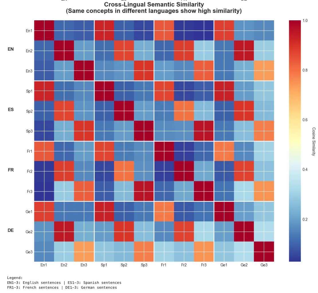
ax.set_title(
'Cross-Lingual Semantic Similarity\n(Same concepts in different languages show high similarity)'
,
fontsize=
16
, fontweight=
'bold'
, pad=
20
)
plt.tight_layout()
plt.show()
# Print legend
print
(
"\nLegend:"
)
print
(
"EN1-3: English sentences | ES1-3: Spanish sentences"
)
print
(
"FR1-3: French sentences | DE1-3: German sentences"
)
print
(
"\n1: Password reset | 2: Customer support | 3: Refund policy"
)
-
Search Hugging Face for domain models (legal, biomedical, financial)
-
Fine-tune base models on your data (see Article 10)
-
Use APIs with strong domain-specific MTEB performance
-
Deploy multilingual models for global reach
-
Adapt models for specialized domains
-
Prefer long-context support for documents
-
Benchmark using MTEB for optimal selection
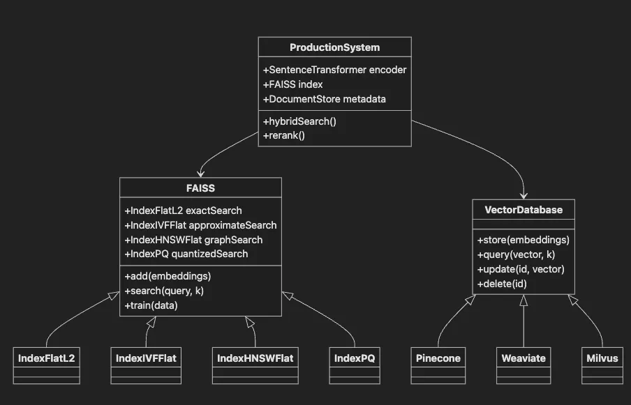
- FAISS base class provides vector search functionality
- Subclasses offer different index types for various use cases
- VectorDatabase interface implemented by managed solutions
- ProductionSystem integrates FAISS with transformers and metadata
- Shows relationships between components in real deployments
# Import necessary libraries
import
 numpy
as
 np
import
 time
import
 faiss
from
 sentence_transformers
import
 SentenceTransformer
import
 matplotlib.pyplot
as
 plt
import
 seaborn
as
 sns
import
 warnings
warnings.filterwarnings(
'ignore'
)
# Set up plotting style
plt.style.use(
'seaborn-v0_8-darkgrid'
)
sns.set_palette(
"husl"
)
print
(
"Libraries imported successfully!"
)
print
(
f"FAISS version:
{faiss.__version__}
"
)
- Import Core Libraries: Load FAISS and supporting packages
- Import Visualization Tools: Set up matplotlib and seaborn for analysis
- Configure Environment: Suppress warnings and set plotting style
- Verify Installation: Print FAISS version to confirm setup
- Ready for Indexing: System prepared for vector operations
# Compare different FAISS index types
import
 time
# Make sure doc_embeddings is defined
if

'doc_embeddings'

not

in

globals
():

print
(
"Please run the previous cell first to generate embeddings!"
)
else
:
    dimension = doc_embeddings.shape[
1
]
    indices = {}
    build_times = {}

# 1. Exact search (IndexFlatL2)
    start = time.time()
    index_flat = faiss.IndexFlatL2(dimension)
    index_flat.add(doc_embeddings)
    build_times[
'Flat L2 (Exact)'
] = time.time() - start
    indices[
'Flat L2 (Exact)'
] = index_flat

# 2. Approximate search (IndexIVFFlat)
    start = time.time()
    nlist =
50

# Number of clusters
    quantizer = faiss.IndexFlatL2(dimension)
    index_ivf = faiss.IndexIVFFlat(quantizer, dimension, nlist)
    index_ivf.train(doc_embeddings)
# Training required
    index_ivf.add(doc_embeddings)
    build_times[
'IVF Flat (Approximate)'
] = time.time() - start
    indices[
'IVF Flat (Approximate)'
] = index_ivf

# 3. Graph-based search (IndexHNSWFlat)
    start = time.time()
    index_hnsw = faiss.IndexHNSWFlat(dimension,
32
)
# 32 is the connectivity parameter
    index_hnsw.add(doc_embeddings)
    build_times[
'HNSW (Graph)'
] = time.time() - start
    indices[
'HNSW (Graph)'
] = index_hnsw

print
(
"Index Build Times:"
)

for
 name, time_taken
in
 build_times.items():

print
(
f"
{name}
:
{time_taken:
.3
f}
 seconds"
)
⚠️ Required data
not
 found.
Let
's create it now...
Generating embeddings...
Batches:

100%

32
/
32
 [
00
:
00
<
00
:
00
,
76.18
it/s]
Generated embeddings
with
 shape: (
1000
,
384
)
Index Build Times:
  Flat L2 (Exact):
0.001
 seconds
  IVF Flat (Approximate):
0.008
 seconds
  HNSW (Graph):
0.006
 seconds
WARNING clustering
1000
 points
to

50
 centroids: please provide at least
1950
 training points
- Get Dimension: Extract embedding vector length (e.g., 384)
- Create Exact Index: Initialize L2 distance index for accurate search
- Build Approximate Index: Create IVF index with clustering for speed
- Train IVF: Learn cluster centers from data
- Create Graph Index: Build HNSW for fast approximate search
# Generate embeddings for all documents
print
(
"Generating embeddings..."
)
doc_embeddings = model.encode(synthetic_docs, batch_size=
32
, show_progress_bar=
True
)
doc_embeddings = doc_embeddings.astype(
'float32'
)
# FAISS requires float32
print
(
f"\nEmbeddings shape:
{doc_embeddings.shape}
"
)
print
(
f"Memory usage:
{doc_embeddings.nbytes /
1024
 /
1024
:
.2
f}
 MB"
)
Generating

embeddings...
Batches:

100
%

32
/32
 [
00
:00<00:00
,
93.
01it/s
]
Embeddings shape:

(1000,

384
)
Memory usage:

1.46

MB
- Generate query embedding (same model as documents)
- Search FAISS index for nearest neighbors
- Map results to original data
# Benchmark search performance
if

'indices'

not

in

globals
()
or

not
 indices:

print
(
"⚠️ Indices not found. Please run the previous cell first to build indices!"
)
elif

'model'

not

in

globals
():

print
(
"⚠️ Model not found. Loading model..."
)
    model = SentenceTransformer(
'all-MiniLM-L6-v2'
)
else
:
    query =
"Looking for AI and machine learning resources"
    query_embedding = model.encode([query]).astype(
'float32'
)
    k =
10

# Number of neighbors
    search_times = {}
    search_results = {}

for
 name, index
in
 indices.items():

# Set search parameters for IVF

if

'IVF'

in
 name:
            index.nprobe =
10

# Number of clusters to search


# Perform search
        start = time.time()
        distances, indices_found = index.search(query_embedding, k)
        search_times[name] = (time.time() - start) *
1000

# Convert to ms
        search_results[name] = (distances[
0
], indices_found[
0
])

# Visualize performance comparison
    fig, (ax1, ax2) = plt.subplots(
1
,
2
, figsize=(
14
,
5
))

# Build times
    names =
list
(build_times.keys())
    build_values =
list
(build_times.values())
    ax1.bar(names, build_values, color=[
'green'
,
'orange'
,
'blue'
])
    ax1.set_title(
'Index Build Time Comparison'
, fontsize=
14
, fontweight=
'bold'
)
    ax1.set_ylabel(
'Time (seconds)'
)
    ax1.tick_params(axis=
'x'
, rotation=
45
)

# Search times
    search_values =
list
(search_times.values())
    ax2.bar(names, search_values, color=[
'green'
,
'orange'
,
'blue'
])
    ax2.set_title(
'Search Time Comparison'
, fontsize=
14
, fontweight=
'bold'
)
    ax2.set_ylabel(
'Time (milliseconds)'
)
    ax2.tick_params(axis=
'x'
, rotation=
45
)
    plt.tight_layout()
    plt.show()

# Display search results

print
(
f"\nQuery: '
{query}
'"
)

print
(
"\nTop 5 results from each index type:"
)

for
 name, (distances, indices_found)
in
 search_results.items():

print
(
f"\n
{name}
:"
)

for
 i
in

range
(
5
):
            idx = indices_found[i]
            dist = distances[i]

print
(
f"
{i+
1
}
.
{synthetic_docs[idx][:
60
]}
... (distance:
{dist:
.3
f}
)"
)
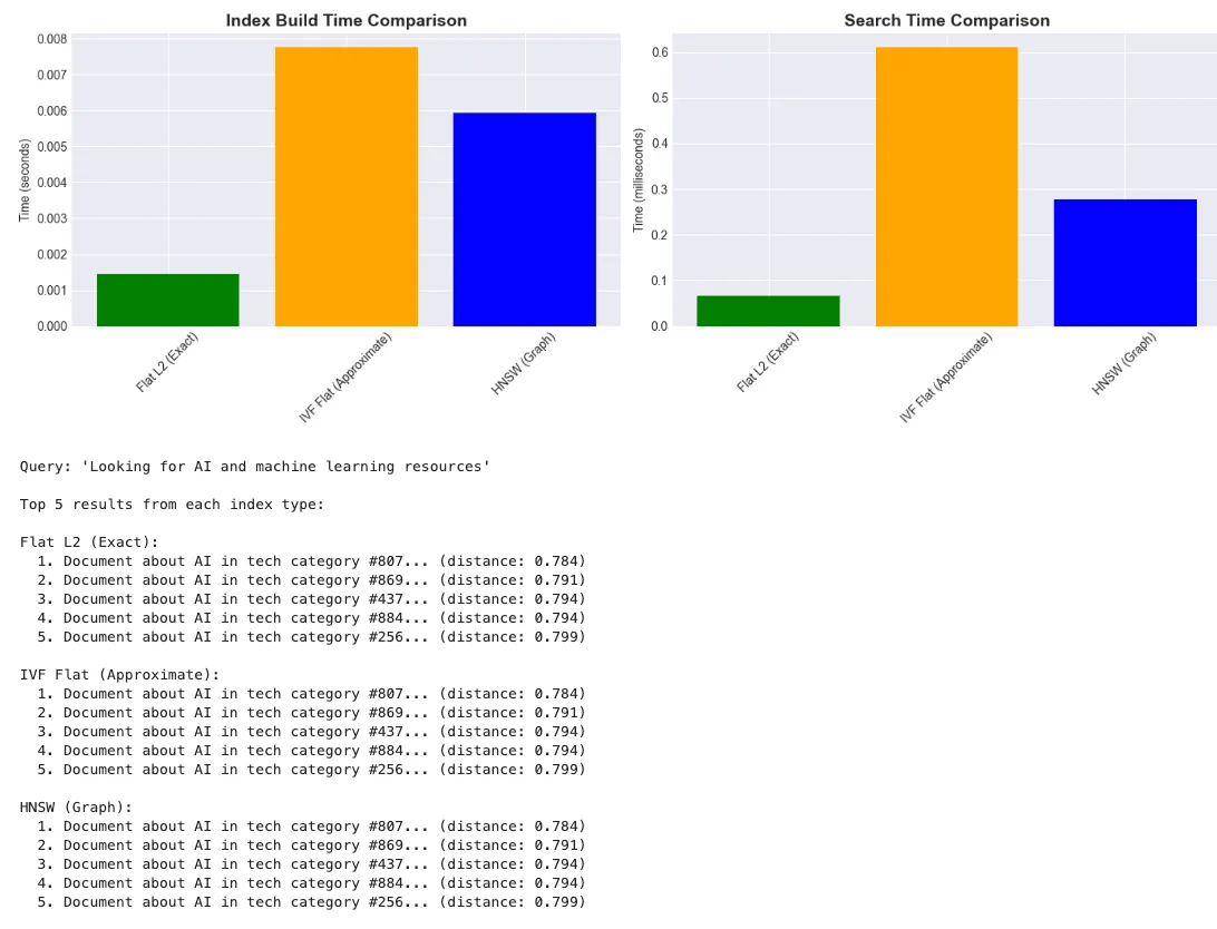
- Define Query: User’s search question
- Generate Embedding: Convert query to vector using same model
- Configure Search: Set parameters for different index types
- Execute Search: Find top-k most similar embeddings
- Measure Performance: Track search time in milliseconds
- Display Results: Show matching documents with distances
# Compare different FAISS index types
dimension = doc_embeddings.shape[1]
indices = {}
build_times = {}
# 1. Exact search (IndexFlatL2)
start = time.time()
index_flat = faiss.IndexFlatL2(dimension)
index_flat.add(doc_embeddings)
build_times['Flat L2 (Exact)'] = time.time() - start
indices['Flat L2 (Exact)'] = index_flat
# 2. Approximate search (IndexIVFFlat)
start = time.time()
nlist = 50
# Number of clusters
quantizer = faiss.IndexFlatL2(dimension)
index_ivf = faiss.IndexIVFFlat(quantizer, dimension, nlist)
index_ivf.train(doc_embeddings)
# Training required
index_ivf.add(doc_embeddings)
build_times['IVF Flat (Approximate)'] = time.time() - start
indices['IVF Flat (Approximate)'] = index_ivf
# 3. Graph-based search (IndexHNSWFlat)
start = time.time()
index_hnsw = faiss.IndexHNSWFlat(dimension, 32)
# 32 is the connectivity parameter
index_hnsw.add(doc_embeddings)
build_times['HNSW (Graph)'] = time.time() - start
indices['HNSW (Graph)'] = index_hnsw
print(
"Index Build Times:"
)
for name, time_taken in build_times.items():
    print(f
"  {name}: {time_taken:.3f} seconds"
)
Index Build Times:
  Flat
L2

(Exact)
:
0.001
 seconds
  IVF
Flat

(Approximate)
:
0.006
 seconds

HNSW

(Graph)
:
0.006
 seconds
WARNING clustering
1000
 points to
50
 centroids: please provide at least
1950
 training points
# Benchmark search performance
query =
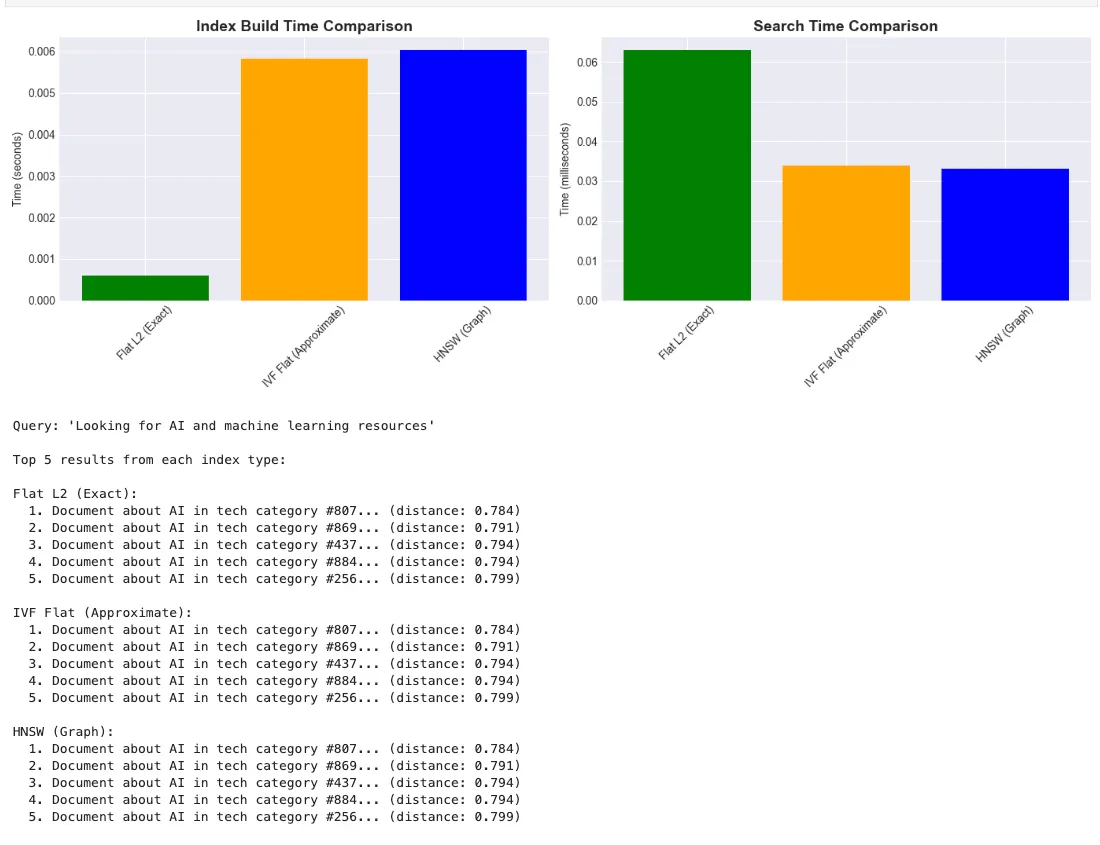
"Looking for AI and machine learning resources"
query_embedding = model.encode([query]).astype(
'float32'
)
k =
10
# Number of neighbors
search_times = {}
search_results = {}
for
name, index
in
indices.items():
# Set search parameters for IVF
if
'IVF'
in
name:
index.nprobe =
10
# Number of clusters to search
# Perform search
start = time.time()
distances, indices_found = index.search(query_embedding, k)
search_times[name] = (time.time() - start) *
1000
# Convert to ms
search_results[name] = (distances[
0
], indices_found[
0
])
# Visualize performance comparison
fig, (ax1, ax2) = plt.subplots(
1
,
2
, figsize=(
14
,
5
))
# Build times
names =
list
(build_times.keys())
build_values =
list
(build_times.values())
ax1.bar(names, build_values, color=[
'green'
,
'orange'
,
'blue'
])
ax1.set_title(
'Index Build Time Comparison'
, fontsize=
14
, fontweight=
'bold'
)
ax1.set_ylabel(
'Time (seconds)'
)
ax1.tick_params(axis=
'x'
, rotation=
45
)
# Search times
search_values =
list
(search_times.values())
ax2.bar(names, search_values, color=[
'green'
,
'orange'
,
'blue'
])
ax2.set_title(
'Search Time Comparison'
, fontsize=
14
, fontweight=
'bold'
)
ax2.set_ylabel(
'Time (milliseconds)'
)
ax2.tick_params(axis=
'x'
, rotation=
45
)
plt.tight_layout()
plt.show()
# Display search results
print
(
f"\nQuery: '
{query}
'"
)
print
(
"\nTop 5 results from each index type:"
)
for
name, (distances, indices_found)
in
search_results.items():
print
(
f"\n
{name}
:"
)
for
i
in
range
(
5
):
idx = indices_found[i]
dist = distances[i]
print
(
f"
{i+
1
}
.
{synthetic_docs[idx][:
60
]}
... (distance:
{dist:
.3
f}
)"
)
# Create a memory-efficient index using Product Quantization
# This reduces memory usage at the cost of some accuracy
# Parameters
nlist =
50

# Number of clusters
m =
8

# Number of subquantizers
nbits =
8

# Bits per subquantizer
# Create index
quantizer = faiss.IndexFlatL2(dimension)
index_pq = faiss.IndexIVFPQ(quantizer, dimension, nlist, m, nbits)
# Train the index
print
(
"Training PQ index..."
)
index_pq.train(doc_embeddings)
index_pq.add(doc_embeddings)
# Compare memory usage
flat_memory = index_flat.ntotal * dimension *
4
 / (
1024
 *
1024
)
# MB
pq_memory = index_pq.ntotal * m * nbits /
8
 / (
1024
 *
1024
)
# MB
print
(
f"\nMemory Usage Comparison:"
)
print
(
f"  Flat Index:
{flat_memory:
.2
f}
 MB"
)
print
(
f"  PQ Index:
{pq_memory:
.2
f}
 MB"
)
print
(
f"  Compression Ratio:
{flat_memory / pq_memory:
.1
f}
x"
)
Training PQ index...
The history saving thread hit an unexpected
error
 (OperationalError(
'attempt to write a readonly database')).History will not be written to the database.
Memory Usage Comparison:
  Flat Index:
1.46
 MB
  PQ Index:
0.01
 MB
  Compression Ratio:
192.0
x
- Define Quantization Parameters: Set clusters, subquantizers, and bits
- Create PQ Index: Combine IVF with product quantization
- Train on Data: Learn quantization codebook
- Add Embeddings: Store compressed representations
- Compare Memory: Show dramatic reduction vs. exact index
# Check if GPU is available for FAISS
gpu_available = faiss.get_num_gpus() >
0
print
(
f"GPU available for FAISS:
{gpu_available}
"
)
if
 gpu_available:

# Create GPU index
    res = faiss.StandardGpuResources()
    index_gpu = faiss.index_cpu_to_gpu(res,
0
, index_flat)


# Benchmark GPU vs CPU
    queries = model.encode([
"test query "
 +
str
(i)
for
 i
in

range
(
100
)]).astype(
'float32'
)


# CPU search
    start = time.time()
    index_flat.search(queries, k)
    cpu_time = time.time() - start


# GPU search
    start = time.time()
    index_gpu.search(queries, k)
    gpu_time = time.time() - start


print
(
f"\nBatch Search Performance (100 queries):"
)

print
(
f"  CPU:
{cpu_time:
.3
f}
 seconds"
)

print
(
f"  GPU:
{gpu_time:
.3
f}
 seconds"
)

print
(
f"  Speedup:
{cpu_time / gpu_time:
.2
f}
x"
)
else
:

print
(
"GPU not available - skipping GPU benchmarks"
)
# Save and load FAISS indices
import
 tempfile
# Create a temporary directory for saving indices
with
 tempfile.TemporaryDirectory()
as
 tmpdir:

# Save index
    index_path = os.path.join(tmpdir,
"faiss_index.bin"
)
    faiss.write_index(index_flat, index_path)

print
(
f"Index saved to:
{index_path}
"
)

print
(
f"File size:
{os.path.getsize(index_path) /
1024
 /
1024
:
.2
f}
 MB"
)


# Load index
    loaded_index = faiss.read_index(index_path)

print
(
f"\nIndex loaded successfully"
)

print
(
f"Number of vectors:
{loaded_index.ntotal}
"
)


# Verify loaded index works
    test_query = model.encode([
"test query"
]).astype(
'float32'
)
    D, I = loaded_index.search(test_query,
5
)

print
(
f"\nTest search on loaded index successful"
)

print
(
f"Top result:
{synthetic_docs[I[
0
][
0
]][:
50
]}
..."
)
Index saved to:

/var/folders/tm/chrvt43s3rbdld20ghw1qtc40000gn/T/tmp69x91c77/faiss_index.bin
File size:

1.46

MB
Index

loaded

successfully
Number of vectors:

1000
Test

search

on

loaded

index

successful
Top result:

Document

about

data

in

tech

category

#52...
# Create a decision guide visualization
fig, ax = plt.subplots(figsize=(
12
,
8
))
# Define index characteristics
index_types = [
'IndexFlatL2'
,
'IndexIVFFlat'
,
'IndexIVFPQ'
,
'IndexHNSWFlat'
]
characteristics = [
'Search Quality'
,
'Search Speed'
,
'Memory Efficiency'
,
'Build Speed'
]
# Scores (1-5 scale)
scores = np.array([
[
5
,
1
,
1
,
5
],
# IndexFlatL2
[
4
,
3
,
3
,
3
],
# IndexIVFFlat
[
3
,
4
,
5
,
2
],
# IndexIVFPQ
[
4
,
5
,
2
,
2
],
# IndexHNSWFlat
])
# Create heatmap
im = ax.imshow(scores.T, cmap=
'RdYlGn'
, aspect=
'auto'
, vmin=
1
, vmax=
5
)
# Set ticks and labels
ax.set_xticks(np.arange(
len
(index_types)))
ax.set_yticks(np.arange(
len
(characteristics)))
ax.set_xticklabels(index_types)
ax.set_yticklabels(characteristics)
# Rotate the tick labels
plt.setp(ax.get_xticklabels(), rotation=
45
, ha=
"right"
, rotation_mode=
"anchor"
)
# Add colorbar
cbar = plt.colorbar(im, ax=ax)
cbar.set_label(
'Score (1=Poor, 5=Excellent)'
, rotation=
270
, labelpad=
20
)
# Add text annotations
for
i
in
range
(
len
(index_types)):
for
j
in
range
(
len
(characteristics)):
text = ax.text(i, j, scores[i, j], ha=
"center"
, va=
"center"
, color=
"black"
)
ax.set_title(
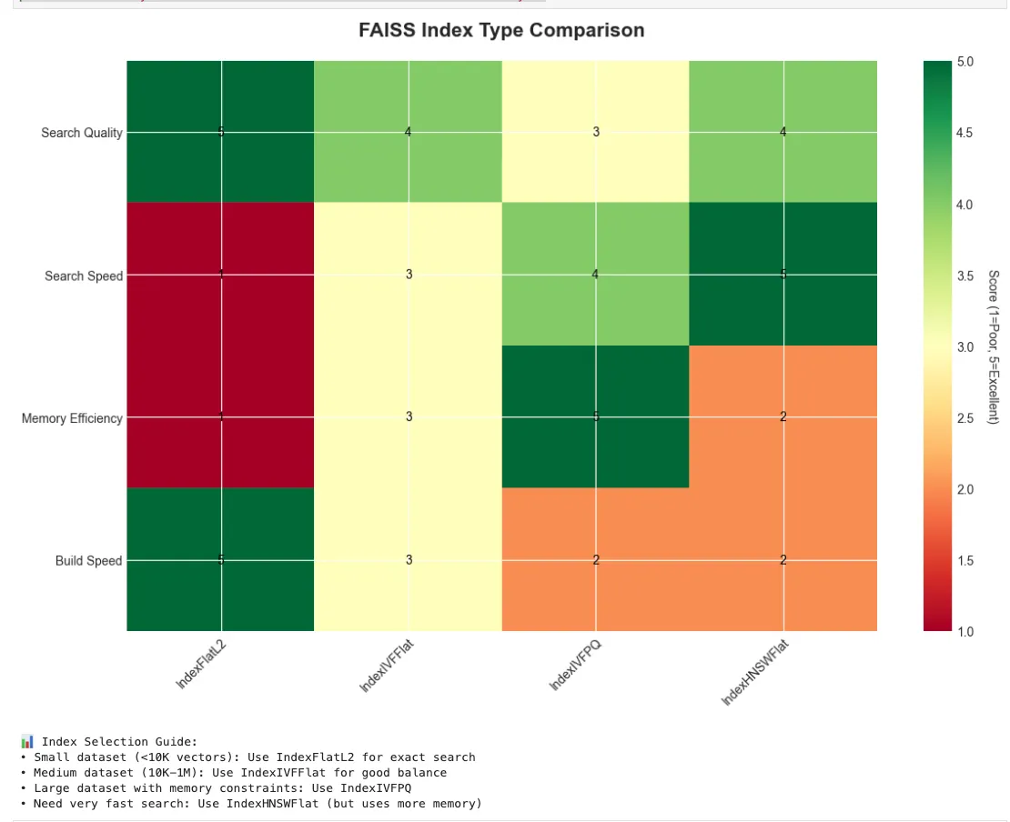
'FAISS Index Type Comparison'
, fontsize=
16
, fontweight=
'bold'
, pad=
20
)
plt.tight_layout()
plt.show()
print
(
"\n📊 Index Selection Guide:"
)
print
(
"• Small dataset (<10K vectors): Use IndexFlatL2 for exact search"
)
print
(
"• Medium dataset (10K-1M): Use IndexIVFFlat for good balance"
)
print
(
"• Large dataset with memory constraints: Use IndexIVFPQ"
)
print
(
"• Need very fast search: Use IndexHNSWFlat (but uses more memory)"
)
# Create a more realistic document search system
class
FAISSDocumentSearch
:
def
__init__
(
self, model_name=
'all-MiniLM-L6-v2'
):
self.model = SentenceTransformer(model_name)
self.index =
None
self.documents = []
def
index_documents
(
self, documents, index_type=
'IVFFlat'
, nlist=
None
):
"""Index documents using specified FAISS index type"""
self.documents = documents
# Generate embeddings
print
(
f"Generating embeddings for
{
len
(documents)}
documents..."
)
embeddings = self.model.encode(documents, show_progress_bar=
True
)
embeddings = embeddings.astype(
'float32'
)
dimension = embeddings.shape[
1
]
n_documents =
len
(documents)
# Auto-adjust nlist if not provided
if
nlist
is
None
:
# Rule of thumb: sqrt(n) clusters, but at least 1 and no more than n_documents
nlist =
max
(
1
,
min
(
int
(np.sqrt(n_documents)), n_documents))
if
index_type ==
'IVFFlat'
:
print
(
f"Auto-adjusted nlist to
{nlist}
based on
{n_documents}
documents"
)
# Create index based on type
if
index_type ==
'Flat'
:
self.index = faiss.IndexFlatL2(dimension)
self.index.add(embeddings)
elif
index_type ==
'IVFFlat'
:
# For small datasets, fall back to Flat index
if
n_documents <
40
:
print
(
f"⚠️ Only
{n_documents}
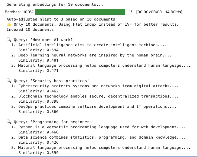
documents. Using Flat index instead of IVF for better results."
)
self.index = faiss.IndexFlatL2(dimension)
self.index.add(embeddings)
else
:
quantizer = faiss.IndexFlatL2(dimension)
self.index = faiss.IndexIVFFlat(quantizer, dimension, nlist)
self.index.train(embeddings)
self.index.add(embeddings)
elif
index_type ==
'HNSW'
:
self.index = faiss.IndexHNSWFlat(dimension,
32
)
self.index.add(embeddings)
print
(
f"Indexed
{self.index.ntotal}
documents"
)
def
search
(
self, query, k=
5
):
"""Search for similar documents"""
# Generate query embedding
query_embedding = self.model.encode([query]).astype(
'float32'
)
# Adjust k if we have fewer documents
k =
min
(k,
len
(self.documents))
# Search
if
hasattr
(self.index,
'nprobe'
):
self.index.nprobe =
10
# For IVF indices
distances, indices = self.index.search(query_embedding, k)
# Format results
results = []
for
dist, idx
in
zip
(distances[
0
], indices[
0
]):
results.append({
'document'
: self.documents[idx],
'distance'
:
float
(dist),
'similarity'
:
1
/ (
1
+
float
(dist))
# Convert distance to similarity
})
return
results
# Create example documents
example_docs = [
"Python is a versatile programming language used for web development."
,
"Machine learning algorithms can predict future trends from historical data."
,
"Natural language processing helps computers understand human language."
,
"Deep learning neural networks are inspired by the human brain."
,
"Data science combines statistics, programming, and domain knowledge."
,
"Cloud computing provides on-demand access to computing resources."
,
"Cybersecurity protects systems and networks from digital attacks."
,
"DevOps practices combine software development and IT operations."
,
"Blockchain technology enables secure, decentralized transactions."
,
"Artificial intelligence aims to create intelligent machines."
]
# Initialize and test the system
search_system = FAISSDocumentSearch()
search_system.index_documents(example_docs, index_type=
'IVFFlat'
)
# Test queries
test_queries = [
"How does AI work?"
,
"Security best practices"
,
"Programming for beginners"
]
for
query
in
test_queries:
print
(
f"\n🔍 Query: '
{query}
'"
)
results = search_system.search(query, k=
3
)
for
i, result
in
enumerate
(results,
1
):
print
(
f"
{i}
.
{result[
'document'
][:
70
]}
..."
)
print
(
f" Similarity:
{result[
'similarity'
]:
.3
f}
"
)
-
Initialize Search System: Create class with model and index storage
-
Generate Document Embeddings: Batch encode all documents
-
Auto-Configure Parameters: Intelligently set index parameters
-
Choose Index Type: Select appropriate index for dataset size
-
Build and Populate Index: Train (if needed) and add embeddings
-
Approximate Nearest Neighbor (ANN) Search
IndexIVFFlat: Inverted File with Flat quantization (requires training)IndexHNSWFlat: Hierarchical Navigable Small World graphs (no training, fast)IndexLSQ: Locally Sensitive Quantization (GPU support in v1.7.2)IndexPQ: Product Quantization for compression
-
Quantization and Compression
-
Sharding and Distributed Search
-
Hybrid Search: Semantic + Keyword
-
Integrating FAISS with Production Systems
- Use FAISS v1.7.2+ for scalable vector search with latest features
- Select exact or approximate indices based on size and latency needs
- Apply quantization for memory efficiency on large datasets
- Save and version indices for reliability
- Integrate with distributed or hybrid search as needed
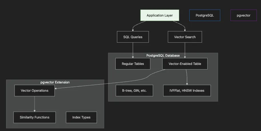
- Application Layer sends both traditional SQL and vector search queries
- PostgreSQL Database contains regular tables and vector-enabled tables
- pgvector Extension provides vector operations and specialized indexes
- Vector Indexes (IVFFlat, HNSW) accelerate similarity search
- Integration allows joining vector results with relational data
- ACID Compliance: Full transactional guarantees for vector operations
- SQL Integration: JOIN vector search results with existing data
- Mature Ecosystem: Leverage PostgreSQL’s tooling, monitoring, backups
- Hybrid Queries: Combine semantic search with filters, aggregations
- Cost Efficiency: Use existing PostgreSQL infrastructure
# Import required libraries
import
 os
import
 psycopg2
from
 psycopg2.extras
import
 RealDictCursor
import
 numpy
as
 np
from
 sentence_transformers
import
 SentenceTransformer
import
 pandas
as
 pd
import
 matplotlib.pyplot
as
 plt
import
 seaborn
as
 sns
import
 time
from
 dotenv
import
 load_dotenv
import
 json
# Load environment variables
load_dotenv()
# Set plotting style
plt.style.use(
'seaborn-v0_8-darkgrid'
)
sns.set_palette(
"husl"
)
print
(
"Libraries imported successfully!"
)
Libraries
 imported successfully!
# Database connection parameters
conn_params = {

'host'
:
os
.
getenv
(
'POSTGRES_HOST'
,
'localhost'
),

'port'
:
os
.
getenv
(
'POSTGRES_PORT'
,
'5433'
),

'dbname'
:
os
.
getenv
(
'POSTGRES_DB'
,
'vector_demo'
),

'user'
:
os
.
getenv
(
'POSTGRES_USER'
,
'postgres'
),

'password'
:
os
.
getenv
(
'POSTGRES_PASSWORD'
,
'postgres'
)
}
# Connect to PostgreSQL
try:
    conn = psycopg2.connect(**conn_params)
    cursor = conn.cursor(cursor_factory=RealDictCursor)

print
(
"✅ Connected to PostgreSQL"
)

    # Register pgvector extension
    from pgvector.psycopg2 import register_vector
    register_vector(conn)

print
(
"✅ pgvector extension registered"
)

except Exception as e:

print
(f
"❌ Connection failed: {e}"
)

print
(
"\nPlease ensure PostgreSQL is running:"
)

print
(
"  task postgres-start"
)
✅ Connected
to
 PostgreSQL
✅ pgvector extension registered
# Enable pgvector extension
cursor.execute(
"CREATE EXTENSION IF NOT EXISTS vector"
)
conn.commit()
print
(
"✅ pgvector extension enabled"
)
# Check version
cursor.execute(
"SELECT extversion FROM pg_extension WHERE extname = 'vector'"
)
version = cursor.fetchone()
print
(
f"pgvector version:
{version[
'extversion'
]
if
 version
else

'Not found'
}
"
)
✅
 pgvector
extension

enabled
pgvector

version
: 0.8.0
# Load sentence transformer model
print
(
"Loading embedding model..."
)
model = SentenceTransformer(
'all-MiniLM-L6-v2'
)
dimension = model.get_sentence_embedding_dimension()
print
(
f"✅ Model loaded (dimension:
{dimension}
)"
)
Loading embedding model...
✅ Model
loaded

(dimension:
384
)
- Import Libraries: Load PostgreSQL adapter and pgvector support
- Configure Connection: Set database connection parameters
- Connect to Database: Establish PostgreSQL connection
- Register pgvector: Enable vector operations in Python
- Handle Errors: Provide helpful error messages if connection fails
# Drop existing table if exists
cursor.execute(
"DROP TABLE IF EXISTS documents CASCADE"
)
# Create table with vector column
create_table_sql =
f"""
CREATE TABLE documents (
    id SERIAL PRIMARY KEY,
    content TEXT NOT NULL,
    embedding vector(
{dimension}
),
    metadata JSONB,
    created_at TIMESTAMP DEFAULT CURRENT_TIMESTAMP
)
"""
cursor.execute(create_table_sql)
conn.commit()
print
(
"✅ Table 'documents' created"
)
# Show table structure
cursor.execute(
"""
    SELECT column_name, data_type
    FROM information_schema.columns
    WHERE table_name = 'documents'
"""
)
columns = cursor.fetchall()
print
(
"\nTable structure:"
)
for
 col
in
 columns:

print
(
f"  -
{col[
'column_name'
]}
:
{col[
'data_type'
]}
"
)
- Enable Extension: Activate pgvector in the database
- Verify Version: Check pgvector installation
- Load Embedding Model: Initialize sentence transformer
- Define Schema: Create table with vector column matching embedding dimensions
- Add Metadata Support: Include JSONB for flexible additional data
# Sample documents
documents = [

"PostgreSQL is a powerful, open source relational database system."
,

"Vector databases enable semantic search using embeddings."
,

"pgvector adds vector similarity search to PostgreSQL."
,

"Machine learning models generate embeddings for text data."
,

"Semantic search understands meaning, not just keywords."
,

"ACID transactions ensure data consistency in databases."
,

"SQL queries can combine vector search with filters."
,

"Embeddings capture semantic relationships between words."
,

"PostgreSQL supports JSON data types natively."
,

"Vector similarity search finds related documents efficiently."
]
# Generate embeddings
print
(
"Generating embeddings..."
)
embeddings = model.encode(documents, show_progress_bar=
True
)
# Insert documents with embeddings
insert_sql =
"""
INSERT INTO documents (content, embedding, metadata)
VALUES (%s, %s, %s)
"""
for
 i, (doc, emb)
in

enumerate
(
zip
(documents, embeddings)):
    metadata = {

'length'
:
len
(doc),

'word_count'
:
len
(doc.split()),

'category'
:
'database'

if

'database'

in
 doc.lower()
else

'ml'
    }
    cursor.execute(insert_sql, (doc, emb.tolist(), json.dumps(metadata)))
conn.commit()
print
(
f"\n✅ Inserted
{
len
(documents)}
 documents"
)
Generating embeddings...
Batches:

0
%|          |

0
/
1
 [
00
:
00
<
?,

?i
t/s]
✅ Inserted
10
 documents
- Define Documents: Create sample texts covering various topics
- Generate Embeddings: Convert documents to vectors
- Prepare Metadata: Add structured information about each document
- Insert with Vectors: Store documents, embeddings, and metadata together
- Commit Transaction: Ensure data is persisted
# Function to perform semantic search
def

semantic_search
(
query, limit=
5
):

# Generate query embedding
    query_embedding = model.encode(query)


# Search using cosine similarity
    search_sql =
"""
    SELECT
        id,
        content,
        1 - (embedding <=> %s::vector) AS similarity,
        metadata
    FROM documents
    ORDER BY embedding <=> %s::vector
    LIMIT %s
    """

    cursor.execute(search_sql, (query_embedding.tolist(), query_embedding.tolist(), limit))

return
 cursor.fetchall()
# Test semantic search
query =
"How to search for similar text?"
print
(
f"🔍 Query: '
{query}
'\n"
)
results = semantic_search(query)
for
 i, result
in

enumerate
(results,
1
):

print
(
f"
{i}
.
{result[
'content'
][:
70
]}
..."
)

print
(
f"   Similarity:
{result[
'similarity'
]:
.3
f}
"
)

print
(
f"   Category:
{result[
'metadata'
][
'category'
]}
\n"
)
🔍

Query:

'How to search for similar text?'
1
.

Vector

similarity

search

finds

related

documents

efficiently....

Similarity:

0.594

Category:

ml
2
.

Semantic

search

understands

meaning,

not

just

keywords....

Similarity:

0.373

Category:

ml
3
.

SQL

queries

can

combine

vector

search

with

filters....

Similarity:

0.354

Category:

ml
4
.

Vector

databases

enable

semantic

search

using

embeddings....

Similarity:

0.329

Category:

database
5
.

pgvector

adds

vector

similarity

search

to

PostgreSQL....

Similarity:

0.320

Category:

ml
- Encode Query: Convert search query to embedding
- Use Cosine Distance: The
<=>operator calculates cosine distance - Convert to Similarity: Use
1 - distancefor intuitive scores - Order by Distance: Sort results by vector similarity
- Return with Metadata: Include document metadata in results
# Test different index types
index_tests = [
    {
"name"
:
"No Index"
,
"create_sql"
:
None
},
    {

"name"
:
"IVFFlat"
,

"create_sql"
:
"CREATE INDEX idx_ivfflat ON documents_test USING ivfflat (embedding vector_cosine_ops) WITH (lists = 50)"
    },
    {

"name"
:
"HNSW"
,

"create_sql"
:
"CREATE INDEX idx_hnsw ON documents_test USING hnsw (embedding vector_cosine_ops) WITH (m = 16, ef_construction = 64)"
    }
]
# Generate test data and compare performance
# Create synthetic documents for testing
large_docs = []
for
 i
in

range
(
1000
):
    cat = np.random.choice(categories)
    word = np.random.choice(templates[cat])
    large_docs.append(
f"Document about
{word}
 in
{cat}
 category #
{i}
"
)
# Generate embeddings in batches
large_embeddings = model.encode(large_docs, batch_size=
32
, show_progress_bar=
True
)
# Test each index type
for
 test
in
 index_tests:

print
(
f"\\\\nTesting
{test[
'name'
]}
..."
)

# Create index if specified

if
 test[
'create_sql'
]:
        cursor.execute(test[
'create_sql'
])
        conn.commit()

# Benchmark searches

# ... performance testing code ...
- Define Index Types: Compare no index, IVFFlat, and HNSW
- IVFFlat Parameters: Set number of lists for clustering
- HNSW Parameters: Configure graph construction parameters
- Generate Test Data: Create larger dataset for meaningful comparison
- Benchmark Performance: Measure index creation and search times
# Generate more test data
print
(
"Generating larger dataset..."
)
np.random.seed(
42
)
# Create synthetic documents
categories = [
'tech'
,
'health'
,
'finance'
,
'education'
,
'travel'
]
templates = {

'tech'
: [
'software'
,
'hardware'
,
'programming'
,
'AI'
,
'data'
],

'health'
: [
'wellness'
,
'medicine'
,
'fitness'
,
'nutrition'
,
'mental'
],

'finance'
: [
'investment'
,
'banking'
,
'budget'
,
'savings'
,
'credit'
],

'education'
: [
'learning'
,
'teaching'
,
'courses'
,
'degree'
,
'skills'
],

'travel'
: [
'vacation'
,
'destination'
,
'flights'
,
'hotels'
,
'adventure'
]
}
large_docs = []
for
 i
in

range
(
1000
):
    cat = np.random.choice(categories)
    word = np.random.choice(templates[cat])
    large_docs.append(
f"Document about
{word}
 in
{cat}
 category #
{i}
"
)
# Generate embeddings in batches
large_embeddings = model.encode(large_docs, batch_size=
32
, show_progress_bar=
True
)
# Insert into a new table for testing
cursor.execute(
"DROP TABLE IF EXISTS documents_test CASCADE"
)
cursor.execute(
f"""
CREATE TABLE documents_test (
    id SERIAL PRIMARY KEY,
    content TEXT,
    embedding vector(
{dimension}
)
)
"""
)
# Bulk insert
print
(
"\nInserting documents..."
)
for
 doc, emb
in

zip
(large_docs, large_embeddings):
    cursor.execute(

"INSERT INTO documents_test (content, embedding) VALUES (%s, %s)"
,
        (doc, emb.tolist())
    )
conn.commit()
print
(
f"✅ Inserted
{
len
(large_docs)}
 documents"
)
Generating

larger

dataset...
Batches:

100
%

32
/32
 [
00
:02<00:00
,
19.
69it/s
]
Inserting

documents...
✅

Inserted

1000
documents
-
Frequently updated data: Better handles insertions and updates without complete rebuilds
-
Memory-constrained environments: Uses less RAM than HNSW
-
Quick index building: Creates indexes faster, especially for large datasets
-
Balanced performance needs: Good compromise between speed, memory, and accuracy
-
Query-intensive workloads: Significantly faster search performance
-
Static or append-only data: Where index rebuilds are infrequent
-
Higher accuracy requirements: Delivers better recall at same k value
-
RAM-rich environments: When memory isn’t a primary constraint
# Test different index types
index_tests = [
    {
"name"
:
"No Index"
,
"create_sql"
:
None
},
    {

"name"
:
"IVFFlat"
,

"create_sql"
:
"CREATE INDEX idx_ivfflat ON documents_test USING ivfflat (embedding vector_cosine_ops) WITH (lists = 50)"
    },
    {

"name"
:
"HNSW"
,

"create_sql"
:
"CREATE INDEX idx_hnsw ON documents_test USING hnsw (embedding vector_cosine_ops) WITH (m = 16, ef_construction = 64)"
    }
]
results = []
test_queries = [
"AI and machine learning"
,
"financial planning"
,
"health and wellness"
]
for
 test
in
 index_tests:

print
(
f"\nTesting
{test[
'name'
]}
..."
)


# Drop all indexes
    cursor.execute(
"DROP INDEX IF EXISTS idx_ivfflat"
)
    cursor.execute(
"DROP INDEX IF EXISTS idx_hnsw"
)


# Create index if specified

if
 test[
'create_sql'
]:
        start = time.time()
        cursor.execute(test[
'create_sql'
])
        conn.commit()
        create_time = time.time() - start

print
(
f"  Index created in
{create_time:
.3
f}
s"
)

else
:
        create_time =
0


# Benchmark searches
    search_times = []

for
 query
in
 test_queries:
        query_emb = model.encode(query)

        start = time.time()
        cursor.execute(
"""
            SELECT content FROM documents_test
            ORDER BY embedding <=> %s::vector
            LIMIT 5
        """
, (query_emb.tolist(),))
        _ = cursor.fetchall()
        search_times.append(time.time() - start)

    avg_search = np.mean(search_times)
    results.append({

'Index Type'
: test[
'name'
],

'Create Time (s)'
: create_time,

'Avg Search (ms)'
: avg_search *
1000
    })

print
(
f"  Avg search time:
{avg_search *
1000
:
.2
f}
ms"
)
# Display results
results_df = pd.DataFrame(results)
display(results_df)
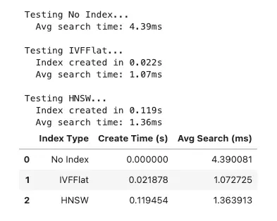
# Create performance visualization
fig, (ax1, ax2) = plt.subplots(1, 2, figsize=(12, 5))
# Index creation time
ax1.bar(results_df[
'Index Type'
], results_df[
'Create Time (s)'
], color=[
'gray'
,
'orange'
,
'blue'
])
ax1.set_title(
'Index Creation Time'
, fontsize=14, fontweight=
'bold'
)
ax1.set_ylabel(
'Time (seconds)'
)
ax1.set_xlabel(
'Index Type'
)
# Search performance
ax2.bar(results_df[
'Index Type'
], results_df[
'Avg Search (ms)'
], color=[
'gray'
,
'orange'
,
'blue'
])
ax2.set_title(
'Average Search Time'
, fontsize=14, fontweight=
'bold'
)
ax2.set_ylabel(
'Time (milliseconds)'
)
ax2.set_xlabel(
'Index Type'
)
plt.tight_layout()
plt.show()
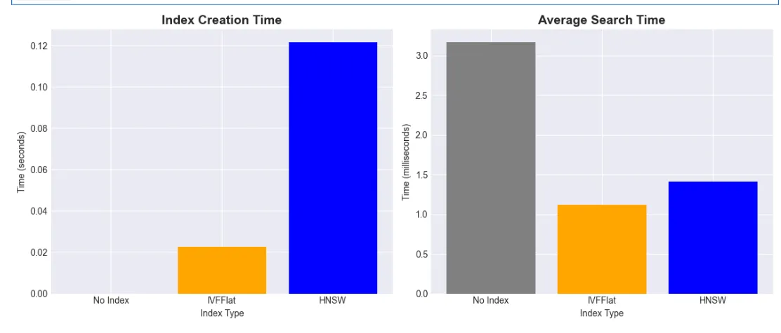
# Demonstrate hybrid search capabilities
print
(
"🔍 Hybrid Search Example\n"
)
# Query 1: Vector search with metadata filter
query =
"database systems"
query_emb = model.encode(query)
hybrid_sql =
"""
SELECT
    content,
    1 - (embedding <=> %s::vector) AS similarity,
    metadata->>'category' AS category,
    metadata->>'word_count' AS word_count
FROM documents
WHERE metadata->>'category' = 'database'
ORDER BY embedding <=> %s::vector
LIMIT 3
"""
cursor.execute(hybrid_sql, (query_emb.tolist(), query_emb.tolist()))
results = cursor.fetchall()
print
(
f"Query: '
{query}
' (filtered by category='database')\n"
)
for
 i, result
in

enumerate
(results,
1
):

print
(
f"
{i}
.
{result[
'content'
][:
60
]}
..."
)

print
(
f"   Similarity:
{result[
'similarity'
]:
.3
f}
"
)

print
(
f"   Words:
{result[
'word_count'
]}
\n"
)
🔍

Hybrid

Search

Example
Query:

'database systems'

(filtered

by

category='database')
1
.

PostgreSQL

is

a

powerful,

open

source

relational

database

sy...

Similarity:

0.658

Words:

9
2
.

ACID

transactions

ensure

data

consistency

in

databases....

Similarity:

0.549

Words:

7
3
.

Vector

databases

enable

semantic

search

using

embeddings....

Similarity:

0.356

Words:

7
-
Combine Vector and SQL: Use WHERE clause with vector search
-
Filter by Metadata: Restrict to specific category
-
Extract JSON Fields: Use ->> operator for JSONB access
-
Order by Similarity: Maintain vector ranking within filtered set
-
Return Rich Results: Include metadata in response
-
Semantic Search with Filtering: The query finds documents semantically similar to a query vector, but only within documents that meet specific criteria
-
Time-Based Filtering: The
WHERE created_at > NOW() - INTERVAL '7 days'clause restricts results to recent documents only -
Metadata Filtering: The
AND metadata->>'category' = 'technical'clause filters by document category using JSON path operators -
Similarity Calculation:
1 - (embedding <=> %s) AS similarityconverts cosine distance to similarity score (0-1 scale) -
Ordering: Results are sorted by vector similarity using the cosine distance operator
<=> -
Result Limiting: Only returns the top 5 most relevant matches
# Compare different distance metrics
query =
"PostgreSQL database"
query_emb = model.encode(query)
metrics_sql =
"""
SELECT
    content,
    embedding <=> %s::vector AS cosine_distance,
    embedding <-> %s::vector AS l2_distance,
    (embedding <#> %s::vector) * -1 AS inner_product
FROM documents
ORDER BY embedding <=> %s::vector
LIMIT 3
"""
cursor.execute(
    metrics_sql,
    (query_emb.tolist(), query_emb.tolist(), query_emb.tolist(), query_emb.tolist())
)
results = cursor.fetchall()
print
(
f"📏 Distance Metrics for '
{query}
':\\\\n"
)
for
 i, result
in

enumerate
(results,
1
):

print
(
f"
{i}
.
{result[
'content'
][:
50
]}
..."
)

print
(
f"   Cosine Distance:
{result[
'cosine_distance'
]:
.4
f}
"
)

print
(
f"   L2 Distance:
{result[
'l2_distance'
]:
.4
f}
"
)

print
(
f"   Inner Product:
{result[
'inner_product'
]:
.4
f}
\\\\n"
)
📏

Distance

Metrics

for

'PostgreSQL database':
1
.

PostgreSQL

is

a

powerful,

open

source

relational

d...

Cosine Distance:

0.2959

L2 Distance:

0.7692

Inner Product:

0.7041
2
.

PostgreSQL

supports

JSON

data

types

natively....

Cosine Distance:

0.4880

L2 Distance:

0.9879

Inner Product:

0.5120
3
.

pgvector

adds

vector

similarity

search

to

PostgreS...

Cosine Distance:

0.6039

L2 Distance:

1.0990

Inner Product:

0.3961
- Cosine Distance (<=>): Normalized, focuses on direction
- Euclidean Distance (<->): Actual distance in vector space
- Inner Product (<#>): Dot product, useful for non-normalized vectors
- Choose Appropriately: Most text embeddings work best with cosine
- Understand Trade-offs: Each metric has specific use cases
-
Advantages: Normalizes for vector magnitude, focusing purely on direction/angle
-
When to use: Most transformer models produce normalized embeddings where cosine distance works best
-
Example use case: Semantic document search, where document length shouldn’t affect relevance
-
Advantages: Intuitive physical distance interpretation
-
When to use: Non-normalized embeddings, image feature vectors, or geometric data
-
Example use case: Facial recognition, image similarity, geographical positioning
-
Advantages: Faster computation, works well with specific ML models
-
When to use: Recommendation systems, when vectors are NOT normalized
-
Example use case: Product recommendations where magnitude encodes relevance/popularity
-
Semantic text search Cosine (<=>) Ignores magnitude differences in text embeddings
-
Image similarity Euclidean (<->) Preserves spatial relationships in feature space
-
Recommendations Inner Product (<#>) Captures preference strength and similarity
-
Pre-normalized vectors Cosine or Euclidean Equivalent when vectors are normalized
-
Non-normalized with magnitude importance Inner Product Considers both direction and magnitude

def

choose_index_type
(
num_vectors, update_frequency
):

"""Recommend pgvector index based on use case"""

if
 num_vectors <
10_000
:

return

"No index needed for small datasets"

elif
 update_frequency ==
"high"
:

return

"IVFFlat - handles updates better"

else
:

return

"HNSW - fastest queries for static data"
- Dataset Size Assessment: For small datasets (under 10,000 vectors), the function recommends skipping indexing entirely, as PostgreSQL can efficiently scan small tables without specialized indexes
- Update Frequency Evaluation: For frequently updated data, IVFFlat is recommended due to its better handling of insertions and modifications
- Default to Performance: For static or infrequently changing datasets, HNSW is recommended for its superior query performance
# Efficient batch insertion
def

batch_insert_embeddings
(
documents, batch_size=
100
):
    embeddings = model.encode(documents, batch_size=
32
)

# Use COPY for fastest insertion

with
 cursor.copy(

"COPY documents (content, embedding) FROM STDIN"
    )
as
 copy:

for
 doc, emb
in

zip
(documents, embeddings):
            copy.write_row([doc, emb.tolist()])
- Batch Processing with Transformer Model: The function processes multiple documents at once, generating embeddings in batches of 32 using a transformer model. This is more efficient than encoding documents one by one.
- PostgreSQL COPY Command: Instead of using individual INSERT statements, the code leverages PostgreSQL’s COPY protocol, which is significantly faster for bulk operations.
- Parallel Data Insertion: The function pairs each document with its corresponding embedding vector and inserts them together in a single operation.
- Vector Format Conversion: The embeddings are converted from NumPy arrays to Python lists using
tolist()to ensure compatibility with the database. - Performance Benefits: This approach can be 10–100x faster than individual inserts when adding large numbers of vectors to a database.
def

rag_search
(
question, context_limit=
3
):

"""
    Retrieval-Augmented Generation using pgvector
    """

# Retrieve relevant documents
    query_emb = model.encode(question)

    rag_sql =
"""
    SELECT
        content,
        1 - (embedding <=> %s::vector) AS similarity
    FROM documents
    ORDER BY embedding <=> %s::vector
    LIMIT %s
    """

    cursor.execute(rag_sql, (query_emb.tolist(), query_emb.tolist(), context_limit))
    results = cursor.fetchall()


# Build context
    context_parts = []

for
 i, result
in

enumerate
(results,
1
):
        context_parts.append(
f"
{i}
.
{result[
'content'
]}
 (Relevance:
{result[
'similarity'
]:
.2
%}
)"
)

    context =
"\n"
.join(context_parts)


# Format for LLM
    prompt =
f"""
Based on the following context, answer the question.
Context:
{context}
Question:
{question}
Answer: [This would be sent to an LLM for generation]
"""


return
 prompt, results
# Test RAG search
question =
"How does pgvector help with semantic search?"
prompt, docs = rag_search(question)
print
(
"🤖 RAG Example\n"
)
print
(
f"Question:
{question}
\n"
)
print
(
"Retrieved Documents:"
)
for
 doc
in
 docs:

print
(
f"-
{doc[
'content'
][:
80
]}
..."
)

print
(
f"  Relevance:
{doc[
'similarity'
]:
.2
%}
\n"
)
print
(
"\nGenerated Prompt (truncated):"
)
print
(prompt[:
500
] +
"..."
)
🤖 RAG Example
Question:
 How does pgvector help
with
 semantic search?
Retrieved Documents:
- pgvector adds vector similarity search
to
 PostgreSQL....
  Relevance:
75.35
%
- Vector databases enable semantic search
using
 embeddings....
  Relevance:
64.05
%
- Semantic search understands meaning,
not
 just keywords....
  Relevance:
60.44
%
Generated Prompt (truncated):
Based
on
 the following context, answer the question.
Context:
1
. pgvector adds vector similarity search
to
 PostgreSQL. (Relevance:
75.35
%)
2
. Vector databases enable semantic search
using
 embeddings. (Relevance:
64.05
%)
3
. Semantic search understands meaning,
not
 just keywords. (Relevance:
60.44
%)
Question:
 How does pgvector help
with
 semantic search?
Answer:
 [This would be sent
to
 an LLM
for
 generation]
...
- Retrieve Relevant Context: Use vector search to find related documents
- Build Structured Context: Format documents with relevance scores
- Create LLM Prompt: Combine context with question
- Enable Generation: Prompt ready for LLM processing
- Ground Responses: Ensure answers based on retrieved facts
# Query 2: Combine with aggregation
print
(
"\n📊 Aggregated Analysis\n"
)
agg_sql =
"""
WITH similarity_scores AS (
    SELECT
        metadata->>'category' AS category,
        1 - (embedding <=> %s::vector) AS similarity
    FROM documents
)
SELECT
    category,
    COUNT(*) as doc_count,
    AVG(similarity) as avg_similarity,
    MAX(similarity) as max_similarity
FROM similarity_scores
GROUP BY category
ORDER BY avg_similarity DESC
"""
query =
"machine learning and AI"
query_emb = model.encode(query)
cursor.execute(agg_sql, (query_emb.tolist(),))
results = cursor.fetchall()
print
(
f"Category analysis for query: '
{query}
'\n"
)
for
 result
in
 results:

print
(
f"Category:
{result[
'category'
]}
"
)

print
(
f"  Documents:
{result[
'doc_count'
]}
"
)

print
(
f"  Avg Similarity:
{result[
'avg_similarity'
]:
.3
f}
"
)

print
(
f"  Max Similarity:
{result[
'max_similarity'
]:
.3
f}
\n"
)
📊

Aggregated

Analysis
Category analysis for query:

'machine learning and AI'
Category:

database

Documents:

3

Avg Similarity:

0.189

Max Similarity:

0.268
Category:

ml

Documents:

7

Avg Similarity:

0.181

Max Similarity:

0.397
# Find documents above similarity threshold
query =
"vector similarity search"
query_emb = model.encode(query)
threshold =
0.7
threshold_sql =
"""
SELECT
    content,
    1 - (embedding <=> %s::vector) AS similarity
FROM documents
WHERE 1 - (embedding <=> %s::vector) > %s
ORDER BY similarity DESC
"""
cursor.execute(threshold_sql, (query_emb.tolist(), query_emb.tolist(), threshold))
results = cursor.fetchall()
print
(
f"🎯 Documents with similarity >
{threshold}
 for '
{query}
':\n"
)
for
 result
in
 results:

print
(
f"•
{result[
'content'
]}
"
)

print
(
f"  Similarity:
{result[
'similarity'
]:
.3
f}
\n"
)
🎯 Documents
with
 similarity
>

0.7

for

'vector similarity search'
:
• Vector similarity
search
 finds related documents efficiently.
  Similarity:
0.794
-
Using ChatGPT, Embeddings, and HyDE to Improve Search Results which I published on Jul 14, 2023 for some insight on how to improve your search results with RAG.
-
Conversation about Document Parsing and RAG (VLOG transcripts) Published on May 2, 2025
-
Stop the Hallucinations: Hybrid Retrieval with BM25, pgvector, embedding rerank, LLM Rubric Rerank… Published on May 1, 2025
-
Speed: Fastest for pure vector ops / Good, with SQL overhead
-
ACID Transactions: No / Yes
-
SQL Integration: No / Native
-
Maintenance: Manual / PostgreSQL tools
-
Scaling: Sharding complexity / Read replicas, partitioning
-
Memory Management: Manual / PostgreSQL buffer management
-
Index Types: More options / IVFFlat, HNSW
-
Updates: Limited / Full CRUD support
from
 psycopg2
import
 pool
# Create connection pool for better performance
connection_pool = pool.SimpleConnectionPool(

1
,
20
,
# min and max connections
    host=
"localhost"
,
    port=
"5433"
,
    database=
"vector_demo"
,
    user=
"postgres"
,
    password=
"postgres"
)
def

search_with_pool
(
query_text
):
    conn = connection_pool.getconn()

try
:

# Perform search

# ...

finally
:
        connection_pool.putconn(conn)
-
Create Pool: Initialize connection pool with min/max connections
-
Get Connection: Obtain connection from pool when needed
-
Use Connection: Perform vector search operations
-
Return Connection: Always return connection to pool
-
Maximize Efficiency: Reuse connections across requests
-
Index Management: Create indexes after bulk loading for faster initial setup
-
Dimension Consistency: Ensure all vectors have the same dimensions
-
Connection Pooling: Use connection pools for concurrent requests
-
Backup Strategy: Regular pg_dump includes vector data automatically
-
Version Control: Track schema changes including vector columns
-
Query Monitoring: Use pg_stat_statements to optimize slow queries
-
Introduction to FTS limitations of pure embeddings — Explaining when and why you need keyword search alongside semantic search
-
PostgreSQL FTS fundamentals — Showing how tsvector works with tokenization, stop-word removal, and stemming
-
Comparison examples — Side-by-side comparison of vector search vs FTS on different query types
-
Hybrid search implementation — A complete hybrid search function that combines both approaches with configurable weights
-
Enhanced RAG system — An advanced RAG implementation that uses adaptive weighting based on query characteristics (technical vs conceptual)
-
Performance comparison — Benchmarking all three approaches to show trade-offs
-
Clear guidance — When to use each approach (vector, FTS, or hybrid)
-
Queries are conceptual or abstract
-
Users may use different terminology than documents
-
You need to find semantically related content
-
Cross-language search is required
-
Exact phrase matching is critical (error codes, technical terms)
-
You need to find specific keywords or identifiers
-
Users know the exact terminology
-
Performance is critical and queries are simple
-
You need the best of both worlds
-
Query patterns are mixed (technical + conceptual)
-
Building a production search system
-
Implementing RAG systems that need both precision and recall
# Add Full-Text Search column to our documents table
print
(
"🔍 Adding Full-Text Search capabilities...\n"
)
# First, let's check if the column already exists
cursor.execute(
"""
    SELECT column_name
    FROM information_schema.columns
    WHERE table_name = 'documents' AND column_name = 'content_tsv'
"""
)
column_exists = cursor.fetchone()
if

not
 column_exists:

# Add tsvector column for FTS
    alter_table_sql =
"""
    ALTER TABLE documents
    ADD COLUMN content_tsv tsvector
    GENERATED ALWAYS AS (to_tsvector('english', content)) STORED;
    """


try
:
        cursor.execute(alter_table_sql)
        conn.commit()

print
(
"✅ Added tsvector column for full-text search"
)

except
 Exception
as
 e:

print
(
f"Error adding column:
{e}
"
)
        conn.rollback()
else
:

print
(
"✅ tsvector column already exists"
)
# Create GIN index for fast text search
create_index_sql =
"""
CREATE INDEX IF NOT EXISTS idx_documents_content_tsv
ON documents USING GIN (content_tsv);
"""
cursor.execute(create_index_sql)
conn.commit()
print
(
"✅ Created/verified GIN index for full-text search"
)
# Verify the column was added
cursor.execute(
"""
    SELECT column_name, data_type
    FROM information_schema.columns
    WHERE table_name = 'documents'
    ORDER BY ordinal_position
"""
)
columns = cursor.fetchall()
print
(
"\nCurrent table structure:"
)
for
 col
in
 columns:

print
(
f"  -
{col[
'column_name'
]}
:
{col[
'data_type'
]}
"
)
# Show what to_tsvector does
print
(
"\n📚 Understanding tsvector transformation:"
)
test_text =
"PostgreSQL is running queries with amazing performance"
cursor.execute(
"SELECT to_tsvector('english', %s) as tsv"
, (test_text,))
result = cursor.fetchone()
print
(
f"\nOriginal: '
{test_text}
'"
)
print
(
f"tsvector:
{result[
'tsv'
]}
"
)
print
(
"\nNotice how:"
)
print
(
"- 'running' becomes 'run' (stemming)"
)
print
(
"- 'is' and 'with' are removed (stop words)"
)
print
(
"- Words are stored with positions for ranking"
)
🔍 Adding
Full
-
Text
Search
 capabilities...
✅ Added tsvector
column

for

full
-
text
search
✅ Created
/
verified GIN index
for

full
-
text
search
Current

table
 structure:

-
 id:
integer

-
 content: text

-
 embedding:
USER
-
DEFINED

-
 metadata: jsonb

-
 created_at:
timestamp

without

time
 zone

-
 content_tsv: tsvector
📚 Understanding tsvector transformation:
Original:
'PostgreSQL is running queries with amazing performance'
tsvector:
'amaz'
:
6

'perform'
:
7

'postgresql'
:
1

'queri'
:
4

'run'
:
3
Notice how:
-

'running'
 becomes
'run'
 (stemming)
-

'is'

and

'with'

are
 removed (stop words)
-
 Words
are
 stored
with
 positions
for
 ranking
def

hybrid_rag_search
(
question, context_limit=
3
, adaptive_weights=
True
):

"""
    Enhanced RAG using hybrid search for better retrieval

    Args:
        question: User's question
        context_limit: Number of documents to retrieve
        adaptive_weights: Automatically adjust weights based on query type
    """

# Determine optimal weights based on query characteristics

if
 adaptive_weights:

# Simple heuristic: technical queries favor FTS, conceptual favor vector
        technical_terms = [
'ACID'
,
'SQL'
,
'JSON'
,
'PostgreSQL'
,
'index'
,
'query'
]
        query_words = question.lower().split()


# Check for technical terms
        has_technical =
any
(term.lower()
in
 question.lower()
for
 term
in
 technical_terms)


# Adjust weights

if
 has_technical:
            vector_weight, fts_weight =
0.4
,
0.6

print
(
f"🔧 Detected technical query - favoring FTS"
)

elif

len
(query_words) <=
3
:
            vector_weight, fts_weight =
0.3
,
0.7

print
(
f"📝 Short query - favoring exact matches"
)

else
:
            vector_weight, fts_weight =
0.7
,
0.3

print
(
f"💭 Conceptual query - favoring semantic search"
)

else
:
        vector_weight, fts_weight =
0.6
,
0.4


print
(
f"\n🤖 Hybrid RAG Search"
)

print
(
f"Question:
{question}
"
)

print
(
f"Weights: Vector=
{vector_weight}
, FTS=
{fts_weight}
\n"
)


# Generate query embedding
    query_emb = model.encode(question)


# Enhanced hybrid search with metadata
    rag_sql =
"""
    WITH vector_scores AS (
        SELECT
            id,
            content,
            metadata,
            1 - (embedding <=> %s::vector) AS vector_similarity
        FROM documents
    ),
    fts_scores AS (
        SELECT
            id,
            ts_rank_cd(content_tsv, plainto_tsquery('english', %s)) AS fts_rank,
            ts_headline('english', content, plainto_tsquery('english', %s),
                       'StartSel=**, StopSel=**') AS headline
        FROM documents
        WHERE content_tsv @@ plainto_tsquery('english', %s)
    ),
    combined AS (
        SELECT
            v.id,
            v.content,
            v.metadata,
            v.vector_similarity,
            COALESCE(f.fts_rank, 0) AS fts_rank,
            f.headline,
            (%s * v.vector_similarity) +
            (%s * LEAST(COALESCE(f.fts_rank, 0) * 10, 1)) AS hybrid_score
        FROM vector_scores v
        LEFT JOIN fts_scores f ON v.id = f.id
    )
    SELECT *
    FROM combined
    ORDER BY hybrid_score DESC
    LIMIT %s
    """

    cursor.execute(rag_sql,
                   (query_emb.tolist(), question, question, question,
                    vector_weight, fts_weight, context_limit))
    results = cursor.fetchall()


# Build enhanced context
    context_parts = []

for
 i, result
in

enumerate
(results,
1
):

# Include highlighted text if available

if
 result[
'headline'
]:
            content = result[
'headline'
]

else
:
            content = result[
'content'
]

        context_parts.append(

f"
{i}
.
{content}
\n"

f"   [Category:
{result[
'metadata'
].get(
'category'
,
'unknown'
)}
, "

f"Relevance:
{result[
'hybrid_score'
]:
.2
%}
]"
        )

    context =
"\n\n"
.join(context_parts)


# Create prompt
    prompt =
f"""Based on the following context from a PostgreSQL documentation, answer the question.
Context:
{context}
Question:
{question}
Please provide a comprehensive answer based on the context above. If the context doesn't contain enough information, indicate what's missing.
Answer:"""


print
(
"Retrieved Documents:"
)

for
 i, result
in

enumerate
(results,
1
):

print
(
f"\n
{i}
.
{result[
'content'
][:
80
]}
..."
)

print
(
f"   Vector Score:
{result[
'vector_similarity'
]:
.3
f}
"
)

print
(
f"   FTS Score:
{result[
'fts_rank'
]:
.3
f}
"
)

print
(
f"   Hybrid Score:
{result[
'hybrid_score'
]:
.3
f}
"
)

if
 result[
'headline'
]
and

'**'

in
 result[
'headline'
]:

print
(
f"   Matched Terms:
{result[
'headline'
]}
"
)


return
 prompt, results
# Test enhanced RAG with different question types
test_questions = [

"What are ACID properties in PostgreSQL?"
,

"How does semantic search work?"
,

"Tell me about JSON support"
,
]
for
 question
in
 test_questions:

print
(
"\n"
 +
"="
*
80
)
    prompt, docs = hybrid_rag_search(question, context_limit=
3
)

print
(
"\n📄 Generated Prompt Preview:"
)

print
(prompt[:
600
] +
"..."
)
================================================================================
🔧

Detected

technical

query

-

favoring

FTS
🤖

Hybrid

RAG

Search
Question:

What

are

ACID

properties

in

PostgreSQL?
Weights:

Vector=0.4,

FTS=0.6
Retrieved Documents:
1
.

ACID

transactions

ensure

data

consistency

in

databases....

Vector Score:

0.543

FTS Score:

0.000

Hybrid Score:

0.217
2
.

PostgreSQL

supports

JSON

data

types

natively....

Vector Score:

0.463

FTS Score:

0.000

Hybrid Score:

0.185
3
.

PostgreSQL

is

a

powerful,

open

source

relational

database

system....

Vector Score:

0.443

FTS Score:

0.000

Hybrid Score:

0.177
📄

Generated Prompt Preview:
Based

on

the

following

context

from

a

PostgreSQL

documentation,

answer

the

question.
Context:
1
.

ACID

transactions

ensure

data

consistency

in

databases.
   [
Category:

database
,
Relevance:

21.71
%
]
2
.

PostgreSQL

supports

JSON

data

types

natively.
   [
Category:

ml
,
Relevance:

18.50
%
]
3
.

PostgreSQL

is

a

powerful,

open

source

relational

database

system.
   [
Category:

database
,
Relevance:

17.71
%
]
Question:

What

are

ACID

properties

in

PostgreSQL?
Please

provide

a

comprehensive

answer

based

on

the

context

above.

If

the

context

doesn't

contain

enough

information,

indicate

what's

missing.
Answer:...
================================================================================
💭

Conceptual

query

-

favoring

semantic

search
🤖

Hybrid

RAG

Search
Question:

How

does

semantic

search

work?
Weights:

Vector=0.7,

FTS=0.3
Retrieved Documents:
1
.

Semantic

search

understands

meaning,

not

just

keywords....

Vector Score:

0.783

FTS Score:

0.000

Hybrid Score:

0.548
2
.

Vector

databases

enable

semantic

search

using

embeddings....

Vector Score:

0.588

FTS Score:

0.000

Hybrid Score:

0.411
3
.

SQL

queries

can

combine

vector

search

with

filters....

Vector Score:

0.424

FTS Score:

0.000

Hybrid Score:

0.297
📄

Generated Prompt Preview:
Based

on

the

following

context

from

a

PostgreSQL

documentation,

answer

the

question.
Context:
1
.

Semantic

search

understands

meaning,

not

just

keywords.
   [
Category:

ml
,
Relevance:

54.82
%
]
2
.

Vector

databases

enable

semantic

search

using

embeddings.
   [
Category:

database
,
Relevance:

41.13
%
]
3
.

SQL

queries

can

combine

vector

search

with

filters.
   [
Category:

ml
,
Relevance:

29.67
%
]
Question:

How

does

semantic

search

work?
Please

provide

a

comprehensive

answer

based

on

the

context

above.

If

the

context

doesn't

contain

enough

information,

indicate

what's

missing.
Answer:...
================================================================================
🔧

Detected

technical

query

-

favoring

FTS
🤖

Hybrid

RAG

Search
Question:

Tell

me

about

JSON

support
Weights:

Vector=0.4,

FTS=0.6
Retrieved Documents:
1
.

PostgreSQL

supports

JSON

data

types

natively....

Vector Score:

0.609

FTS Score:

0.000

Hybrid Score:

0.244
2
.

PostgreSQL

is

a

powerful,

open

source

relational

database

system....

Vector Score:

0.223

FTS Score:

0.000

Hybrid Score:

0.089
3
.

ACID

transactions

ensure

data

consistency

in

databases....

Vector Score:

0.217

FTS Score:

0.000

Hybrid Score:

0.087
📄

Generated Prompt Preview:
Based

on

the

following

context

from

a

PostgreSQL

documentation,

answer

the

question.
Context:
1
.

PostgreSQL

supports

JSON

data

types

natively.
   [
Category:

ml
,
Relevance:

24.38
%
]
2
.

PostgreSQL

is

a

powerful,

open

source

relational

database

system.
   [
Category:

database
,
Relevance:

8.92
%
]
3
.

ACID

transactions

ensure

data

consistency

in

databases.
   [
Category:

database
,
Relevance:

8.68
%
]
Question:

Tell

me

about

JSON

support
Please

provide

a

comprehensive

answer

based

on

the

context

above.

If

the

context

doesn't

contain

enough

information,

indicate

what's

missing.
Answer:...
def

hybrid_search
(
query, vector_weight=
0.7
, fts_weight=
0.3
, limit=
5
):

"""
    Hybrid search combining vector similarity and full-text search

    Args:
        query: Search query
        vector_weight: Weight for semantic similarity (0-1)
        fts_weight: Weight for full-text search (0-1)
        limit: Number of results to return
    """

print
(
f"\n🔍 Hybrid Search: '
{query}
'"
)

print
(
f"   Weights: Vector=
{vector_weight}
, FTS=
{fts_weight}
\n"
)


# Generate query embedding
    query_emb = model.encode(query)


# Hybrid search SQL combining both scores
    hybrid_sql =
"""
    WITH vector_scores AS (
        SELECT
            id,
            content,
            1 - (embedding <=> %s::vector) AS vector_similarity
        FROM documents
    ),
    fts_scores AS (
        SELECT
            id,
            ts_rank_cd(content_tsv, plainto_tsquery('english', %s)) AS fts_rank
        FROM documents
        WHERE content_tsv @@ plainto_tsquery('english', %s)
    ),
    combined_scores AS (
        SELECT
            v.id,
            v.content,
            v.vector_similarity,
            COALESCE(f.fts_rank, 0) AS fts_rank,
            -- Normalize FTS rank to 0-1 range (approximate)
            CASE
                WHEN COALESCE(f.fts_rank, 0) = 0 THEN 0
                ELSE LEAST(COALESCE(f.fts_rank, 0) * 10, 1)
            END AS fts_normalized,
            -- Calculate hybrid score
            (%s * v.vector_similarity) +
            (%s * LEAST(COALESCE(f.fts_rank, 0) * 10, 1)) AS hybrid_score
        FROM vector_scores v
        LEFT JOIN fts_scores f ON v.id = f.id
    )
    SELECT
        content,
        vector_similarity,
        fts_normalized,
        hybrid_score
    FROM combined_scores
    ORDER BY hybrid_score DESC
    LIMIT %s
    """

    cursor.execute(hybrid_sql,
                   (query_emb.tolist(), query, query, vector_weight, fts_weight, limit))
    results = cursor.fetchall()


for
 i, result
in

enumerate
(results,
1
):

print
(
f"
{i}
.
{result[
'content'
][:
60
]}
..."
)

print
(
f"   Vector Score:
{result[
'vector_similarity'
]:
.3
f}
"
)

print
(
f"   FTS Score:
{result[
'fts_normalized'
]:
.3
f}
"
)

print
(
f"   Hybrid Score:
{result[
'hybrid_score'
]:
.3
f}
"
)

print
()


return
 results
# Test hybrid search with different weight configurations
test_configs = [
    (
"semantic understanding"
,
0.8
,
0.2
),
# Favor semantic
    (
"ACID transactions"
,
0.5
,
0.5
),
# Balanced
    (
"PostgreSQL"
,
0.3
,
0.7
),
# Favor exact match
]
for
 query, vec_w, fts_w
in
 test_configs:
    hybrid_search(query, vec_w, fts_w, limit=
3
)

print
(
"="
*
60
)
🔍

Hybrid Search:

'semantic understanding'

Weights:

Vector=0.8,

FTS=0.2
1
.

Semantic

search

understands

meaning

and

context,

not

just

ke...

Vector Score:

0.589

FTS Score:

0.500

Hybrid Score:

0.571
2
.

Hybrid

search

combines

keyword

matching

with

semantic

unders...

Vector Score:

0.447

FTS Score:

1.000

Hybrid Score:

0.557
3
.

Embeddings

capture

semantic

relationships

between

words

and

...

Vector Score:

0.454

FTS Score:

0.000

Hybrid Score:

0.364
============================================================
🔍

Hybrid Search:

'ACID transactions'

Weights:

Vector=0.5,

FTS=0.5
1
.

ACID

transactions

ensure

data

consistency

in

databases.

ACID...

Vector Score:

0.686

FTS Score:

1.000

Hybrid Score:

0.843
2
.

Database

consistency

is

maintained

through

ACID

properties

a...

Vector Score:

0.494

FTS Score:

0.333

Hybrid Score:

0.413
3
.

PostgreSQL

is

a

powerful,

open

source

relational

database

sy...

Vector Score:

0.401

FTS Score:

0.000

Hybrid Score:

0.200
============================================================
🔍

Hybrid Search:

'PostgreSQL'

Weights:

Vector=0.3,

FTS=0.7
1
.

PostgreSQL

is

a

powerful,

open

source

relational

database

sy...

Vector Score:

0.678

FTS Score:

1.000

Hybrid Score:

0.903
2
.

PostgreSQL

supports

JSON

data

types

natively

with

JSONB

for

...

Vector Score:

0.561

FTS Score:

1.000

Hybrid Score:

0.868
3
.

pgvector

adds

vector

similarity

search

capabilities

to

Postg...

Vector Score:

0.499

FTS Score:

1.000

Hybrid Score:

0.850
============================================================
- Vector search for semantic understanding
- Full-text search for exact matches
- Weighted scoring to balance both approaches
# Compare Vector Search and Full-Text Search
def

compare_search_methods
(
query
):

"""Compare results from vector search and FTS"""

print
(
f"\n🔍 Query: '
{query}
'\n"
)


# 1. Vector Search

print
(
"=== VECTOR SEARCH (Semantic) ==="
)
    query_emb = model.encode(query)

    vector_sql =
"""
    SELECT
        content,
        1 - (embedding <=> %s::vector) AS similarity
    FROM documents
    ORDER BY embedding <=> %s::vector
    LIMIT 3
    """

    cursor.execute(vector_sql, (query_emb.tolist(), query_emb.tolist()))
    vector_results = cursor.fetchall()


for
 i, result
in

enumerate
(vector_results,
1
):

print
(
f"
{i}
.
{result[
'content'
][:
60
]}
..."
)

print
(
f"   Similarity:
{result[
'similarity'
]:
.3
f}
"
)


# 2. Full-Text Search

print
(
"\n=== FULL-TEXT SEARCH (Lexical) ==="
)


# Convert query to tsquery
    fts_sql =
"""
    SELECT
        content,
        ts_rank_cd(content_tsv, plainto_tsquery('english', %s)) AS rank
    FROM documents
    WHERE content_tsv @@ plainto_tsquery('english', %s)
    ORDER BY rank DESC
    LIMIT 3
    """

    cursor.execute(fts_sql, (query, query))
    fts_results = cursor.fetchall()


if
 fts_results:

for
 i, result
in

enumerate
(fts_results,
1
):

print
(
f"
{i}
.
{result[
'content'
][:
60
]}
..."
)

print
(
f"   Rank:
{result[
'rank'
]:
.3
f}
"
)

else
:

print
(
"   No exact matches found"
)


return
 vector_results, fts_results
# Test with different query types
test_queries = [

"How does PostgreSQL handle ACID transactions?"
,
# Technical query

"database consistency"
,
# Concept query

"JSON data types"
,
# Exact feature query
]
for
 query
in
 test_queries:
    compare_search_methods(query)

print
(
"\n"
 +
"="
*
60
)
🔍 Query:
'How does PostgreSQL handle ACID transactions?'
=
=
=
 VECTOR
SEARCH
 (Semantic)
=
=
=
1.
 ACID transactions ensure data consistency
in
 databases. ACID...
   Similarity:
0.651
2.
 PostgreSQL
is
 a powerful,
open
 source relational database sy...
   Similarity:
0.612
3.
 Database consistency
is
 maintained through ACID properties a...
   Similarity:
0.524
=
=
=

FULL
-
TEXT
SEARCH
 (Lexical)
=
=
=

No
 exact
matches
 found
=
=
=
=
=
=
=
=
=
=
=
=
=
=
=
=
=
=
=
=
=
=
=
=
=
=
=
=
=
=
=
=
=
=
=
=
=
=
=
=
=
=
=
=
=
=
=
=
=
=
=
=
=
=
=
=
=
=
=
=
🔍 Query:
'database consistency'
=
=
=
 VECTOR
SEARCH
 (Semantic)
=
=
=
1.
 Database consistency
is
 maintained through ACID properties a...
   Similarity:
0.760
2.
 ACID transactions ensure data consistency
in
 databases. ACID...
   Similarity:
0.520
3.
 PostgreSQL
is
 a powerful,
open
 source relational database sy...
   Similarity:
0.447
=
=
=

FULL
-
TEXT
SEARCH
 (Lexical)
=
=
=
1.
 Database consistency
is
 maintained through ACID properties a...
   Rank:
0.100
2.
 ACID transactions ensure data consistency
in
 databases. ACID...
   Rank:
0.070
=
=
=
=
=
=
=
=
=
=
=
=
=
=
=
=
=
=
=
=
=
=
=
=
=
=
=
=
=
=
=
=
=
=
=
=
=
=
=
=
=
=
=
=
=
=
=
=
=
=
=
=
=
=
=
=
=
=
=
=
🔍 Query:
'JSON data types'
=
=
=
 VECTOR
SEARCH
 (Semantic)
=
=
=
1.
 PostgreSQL supports JSON data types natively
with
 JSONB
for
 ...
   Similarity:
0.694
2.
 JSON support
in
 PostgreSQL includes operators
for
 querying n...
   Similarity:
0.563
3.
 PostgreSQL
is
 a powerful,
open
 source relational database sy...
   Similarity:
0.243
=
=
=

FULL
-
TEXT
SEARCH
 (Lexical)
=
=
=
1.
 PostgreSQL supports JSON data types natively
with
 JSONB
for
 ...
   Rank:
0.100
=
=
=
=
=
=
=
=
=
=
=
=
=
=
=
=
=
=
=
=
=
=
=
=
=
=
=
=
=
=
=
=
=
=
=
=
=
=
=
=
=
=
=
=
=
=
=
=
=
=
=
=
=
=
=
=
=
=
=
=
# Add Full-Text Search column to our documents table
print
(
"🔍 Adding Full-Text Search capabilities...\n"
)
# Add tsvector column for FTS
alter_table_sql =
"""
ALTER TABLE documents
ADD COLUMN content_tsv tsvector
GENERATED ALWAYS AS (to_tsvector('english', content)) STORED;
"""
try
:
    cursor.execute(alter_table_sql)
    conn.commit()

print
(
"✅ Added tsvector column for full-text search"
)
except
 Exception
as
 e:

print
(
f"Column might already exist:
{e}
"
)
    conn.rollback()
# Create GIN index for fast text search
create_index_sql =
"""
CREATE INDEX IF NOT EXISTS idx_documents_content_tsv
ON documents USING GIN (content_tsv);
"""
cursor.execute(create_index_sql)
conn.commit()
print
(
"✅ Created GIN index for full-text search"
)
# Show what to_tsvector does
print
(
"\n📚 Understanding tsvector transformation:"
)
test_text =
"PostgreSQL is running queries with amazing performance"
cursor.execute(
"SELECT to_tsvector('english', %s) as tsv"
, (test_text,))
result = cursor.fetchone()
print
(
f"\nOriginal: '
{test_text}
'"
)
print
(
f"tsvector:
{result[
'tsv'
]}
"
)
print
(
"\nNotice how:"
)
print
(
"- 'running' becomes 'run' (stemming)"
)
print
(
"- 'is' and 'with' are removed (stop words)"
)
print
(
"- Words are stored with positions for ranking"
)
🔍 Adding
Full
-
Text
Search
 capabilities...
Column
 might already exist:
column
 "content_tsv"
of
 relation "documents" already
exists
✅ Created GIN index
for

full
-
text
search
📚 Understanding tsvector transformation:
Original:
'PostgreSQL is running queries with amazing performance'
tsvector:
'amaz'
:
6

'perform'
:
7

'postgresql'
:
1

'queri'
:
4

'run'
:
3
Notice how:
-

'running'
 becomes
'run'
 (stemming)
-

'is'

and

'with'

are
 removed (stop words)
-
 Words
are
 stored
with
 positions
for
 ranking
- Miss exact phrases (“ACID compliance,”
org.postgresql.Driver) - Struggle with rare tokens (internal code names, SKUs, error codes)
- Over-prioritize feel over facts (returning broad background instead of the line you need)
-
Tokenizes: Breaks text into words
-
Removes stop-words: Filters out “the,” “and,” “is,” etc.
-
Stems words: Reduces words to root form (“running” → “run”)
-
Stores positions: Enables relevance ranking
-
ACID Compliance: Full transactional support for vector operations
-
SQL Integration: Combine semantic search with filters, joins, and aggregations
-
Mature Ecosystem: Leverage existing PostgreSQL tools and infrastructure
-
Flexibility: Choose between different index types based on your needs
-
You need ACID transactions
-
You want to combine vector search with SQL queries
-
You have existing PostgreSQL infrastructure
-
You need full CRUD operations on vectors
-
You need maximum search performance
-
You’re working with billions of vectors
-
You don’t need transactional guarantees
-
You want more index options and GPU support
# Benchmark different embedding models
models_to_test = {

'all-MiniLM-L6-v2'
: {
'dim'
:
384
,
'description'
:
'Fast, lightweight'
},

'all-mpnet-base-v2'
: {
'dim'
:
768
,
'description'
:
'Higher quality, slower'
}
}
# Test documents
test_docs = [
"Sample document "
 +
str
(i)
for
 i
in

range
(
100
)]
benchmark_results = []
for
 model_name, info
in
 models_to_test.items():

print
(
f"\nTesting
{model_name}
..."
)
    test_model = SentenceTransformer(model_name)


# Measure encoding time
    start_time = time.time()
    embeddings = test_model.encode(test_docs, show_progress_bar=
False
)
    encoding_time = time.time() - start_time


# Measure search time
    query_emb = test_model.encode(
"Sample query"
)
    start_time = time.time()
    similarities = util.cos_sim(query_emb, embeddings)
    search_time = time.time() - start_time

    benchmark_results.append({

'Model'
: model_name,

'Dimension'
: info[
'dim'
],

'Description'
: info[
'description'
],

'Encoding Time (ms/doc)'
: (encoding_time /
len
(test_docs)) *
1000
,

'Search Time (ms)'
: search_time *
1000
,

'Memory (MB)'
: embeddings.nbytes /
1024
 /
1024
    })
# Create comparison table
benchmark_df = pd.DataFrame(benchmark_results)
print
(
"\n📊 Model Performance Comparison:"
)
display(benchmark_df)
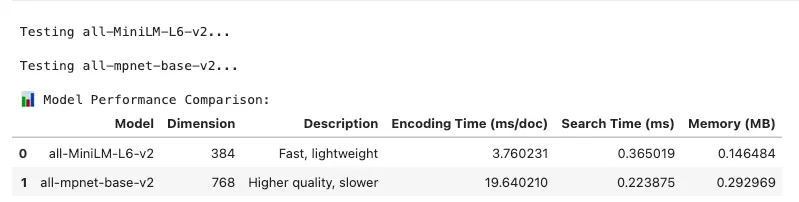
- Define Test Models: Compare lightweight vs. higher-quality models
- Generate Test Data: Create consistent dataset for benchmarking
- Measure Encoding Speed: Time to generate embeddings
- Measure Search Speed: Time to find similar vectors
- Calculate Resource Usage: Track memory consumption
# Visualize performance metrics
fig, axes = plt.subplots(2, 2, figsize=(12, 10))
# Encoding speed
axes[0, 0].bar(benchmark_df[
'Model'
], benchmark_df[
'Encoding Time (ms/doc)'
],
               color=[
'coral'
,
'skyblue'
])
axes[0, 0].set_title(
'Encoding Speed'
, fontsize=12, fontweight=
'bold'
)
axes[0, 0].set_ylabel(
'Time (ms per document)'
)
axes[0, 0].tick_params(axis=
'x'
, rotation=15)
# Search speed
axes[0, 1].bar(benchmark_df[
'Model'
], benchmark_df[
'Search Time (ms)'
],
               color=[
'coral'
,
'skyblue'
])
axes[0, 1].set_title(
'Search Speed'
, fontsize=12, fontweight=
'bold'
)
axes[0, 1].set_ylabel(
'Time (ms)'
)
axes[0, 1].tick_params(axis=
'x'
, rotation=15)
# Memory usage
axes[1, 0].bar(benchmark_df[
'Model'
], benchmark_df[
'Memory (MB)'
],
               color=[
'coral'
,
'skyblue'
])
axes[1, 0].set_title(
'Memory Usage'
, fontsize=12, fontweight=
'bold'
)
axes[1, 0].set_ylabel(
'Memory (MB)'
)
axes[1, 0].tick_params(axis=
'x'
, rotation=15)
# Dimension comparison
axes[1, 1].bar(benchmark_df[
'Model'
], benchmark_df[
'Dimension'
],
               color=[
'coral'
,
'skyblue'
])
axes[1, 1].set_title(
'Embedding Dimension'
, fontsize=12, fontweight=
'bold'
)
axes[1, 1].set_ylabel(
'Dimensions'
)
axes[1, 1].tick_params(axis=
'x'
, rotation=15)
plt.suptitle(
'Embedding Model Performance Comparison'
, fontsize=16, fontweight=
'bold'
)
plt.tight_layout()
plt.show()
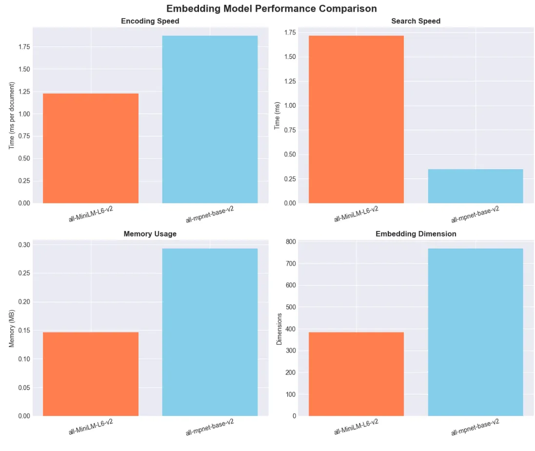
# Create a decision guide visualization
fig, ax = plt.subplots(figsize=(
12
,
8
))
# Define index characteristics
index_types = [
'IndexFlatL2'
,
'IndexIVFFlat'
,
'IndexIVFPQ'
,
'IndexHNSWFlat'
]
characteristics = [
'Search Quality'
,
'Search Speed'
,
'Memory Efficiency'
,
'Build Speed'
]
# Scores (1-5 scale)
scores = np.array([
    [
5
,
1
,
1
,
5
],
# IndexFlatL2
    [
4
,
3
,
3
,
3
],
# IndexIVFFlat
    [
3
,
4
,
5
,
2
],
# IndexIVFPQ
    [
4
,
5
,
2
,
2
],
# IndexHNSWFlat
])
# Create heatmap
im = ax.imshow(scores.T, cmap=
'RdYlGn'
, aspect=
'auto'
, vmin=
1
, vmax=
5
)
# Set ticks and labels
ax.set_xticks(np.arange(
len
(index_types)))
ax.set_yticks(np.arange(
len
(characteristics)))
ax.set_xticklabels(index_types)
ax.set_yticklabels(characteristics)
# Rotate the tick labels
plt.setp(ax.get_xticklabels(), rotation=
45
, ha=
"right"
, rotation_mode=
"anchor"
)
# Add colorbar
cbar = plt.colorbar(im, ax=ax)
cbar.set_label(
'Score (1=Poor, 5=Excellent)'
, rotation=
270
, labelpad=
20
)
# Add text annotations
for
 i
in

range
(
len
(index_types)):

for
 j
in

range
(
len
(characteristics)):
        text = ax.text(i, j, scores[i, j], ha=
"center"
, va=
"center"
, color=
"black"
)
ax.set_title(
'FAISS Index Type Comparison'
, fontsize=
16
, fontweight=
'bold'
, pad=
20
)
plt.tight_layout()
plt.show()
print
(
"\\\\n📊 Index Selection Guide:"
)
print
(
"• Small dataset (<10K vectors): Use IndexFlatL2 for exact search"
)
print
(
"• Medium dataset (10K-1M): Use IndexIVFFlat for good balance"
)
print
(
"• Large dataset with memory constraints: Use IndexIVFPQ"
)
print
(
"• Need very fast search: Use IndexHNSWFlat (but uses more memory)"
)
- Create Visual Guide: Compare index types across key metrics
- Score Characteristics: Rate each index on important factors
- Display Heatmap: Visualize trade-offs clearly
- Provide Recommendations: Guide index selection by use case
- Support Decision Making: Help choose optimal index type
-
✓ Semantic search retrieves by meaning and context, not keywords
-
✓ Transformers and embeddings represent text as semantic vectors
-
✓ FAISS and vector databases enable scalable similarity search
-
✓ Hybrid retrieval combines dense and sparse methods
-
✓ RAG integrates search with LLMs for advanced applications
-
✓ Mastery enables fine-tuning, deployment, and continuous improvement
-
Semantic Search: Finds results based on meaning and context
-
Embedding: Dense vector capturing semantic meaning
-
Sentence Transformer: Model generating sentence-level embeddings
-
FAISS: Library for fast, scalable vector similarity search
-
Vector Database: Managed system for storing/querying embeddings at scale
-
Hybrid Search: Combines semantic and keyword retrieval
-
RAG: Retrieval-Augmented Generation for context-aware LLM answers
-
Precision/Recall: Metrics evaluating search quality
- Hugging Faces Transformers and the AI Revolution (Article 1)
- Hugging Faces: Why Language is Hard for AI? How Transformers Changed that (Article 2)
- Hands-On with Hugging Face: Building Your AI Workspace (Article 3)
- Inside the Transformer: Architecture and Attention Demystified (Article 4)
- Tokenization: The Gateway to Transformer Understanding (Article 5)
- Prompt Engineering (Article 6)
- Extending Transformers Beyond Language (Article 7)
- Customizing Pipelines and Data Workflows: Advanced Models and Efficient Processing (Article 8)
-
Medium Series: Beyond Language: Transformers for Vision, Audio, and Multimodal AI — Article 7 — Extend semantic search to multimodal data.
-
The Economics of Deploying Large Language Models: Costs, Value, and 99.7% Savings — Optimize semantic systems for enterprise scale.
-
Blog Insights: Revolutionizing AI Reasoning: How Reinforcement Learning and GRPO Transform LLMs — Enhance search with advanced reasoning.
-
Building Custom Language Models: From Raw Data to AI Solutions — Curate data for better embeddings.
-
Words as Code: How Prompt Engineering Is Reshaping AI’s Business Impact — Query optimization for semantic systems.
-
Embedding Generation: Create semantic embeddings with multiple models (local and API-based)
-
Hybrid Search: Combine keyword (BM25) and semantic search for optimal results
-
Vector Databases: Implement scalable search with FAISS and Chroma
-
RAG Systems: Build Retrieval-Augmented Generation pipelines
-
Production Patterns: Real-world deployment strategies and optimizations
-
Model Optimization: Quantization techniques for efficient deployment
-
Python 3.12 (managed via pyenv)
-
Poetry for dependency management
-
Go Task for build automation
-
API keys for any required services (see .env.example)
- Clone this repository
git
clone
 [email protected]:RichardHightower/art_hug_09.git
task setup
.
├── src/
│   ├── __init__.py
│   ├── config.py
# Configuration and utilities
│   ├── main.py
# Entry point with all examples
│   ├── embedding_generation.py
# Generate embeddings with many models
│   ├── hybrid_search.py
# Hybrid keyword + semantic search
│   ├── vector_db_manager.py
# FAISS and Chroma database management
│   ├── rag_integration.py
# RAG pipeline implementation
│   └── utils.py
# Utility functions
├── tests/
│   └── test_examples.py
# Unit tests
├── docs/
│   ├── article9.md
# Original article
│   └── article9i.md
# Enhanced article with additional examples
├── notebooks/
│   ├── tutorial.ipynb
# Interactive tutorial
│   ├── faiss_vector_db.ipynb
# FAISS examples
│   └── postgres_vector_db.ipynb
# PostgreSQL pgvector examples
├── .env.example
# Environment template
├── Taskfile.yml
# Task automation
└── pyproject.toml
# Poetry configuration
task run
task run-embeddings
# Generate embeddings with various models
task run-hybrid
# Run hybrid search examples
task run-vector-db
# Vector database management
task run-rag
# Run RAG implementation
task run-quantization
# Run quantization examples
task postgres-logs
# View PostgreSQL logs
task postgres-shell
# Connect to PostgreSQL shell
task postgres-start
# Start PostgreSQL with pgvector extension
task postgres-stop
# Stop PostgreSQL container
python src/main.py
# Choose examples interactively
task notebook
# Launch in Jupyter Notebook
# or
task notebook-lab
# Launch in JupyterLab
# or
# To see FAISS Notebook and Postgres Notebook run this
task notebooks
- Interactive comparisons of keyword vs. semantic search
- Visualizations of embeddings and similarity matrices
- Real-time performance benchmarking
- Hands-on exercises to build your own search systems
- Step-by-step explanations with expected results
%

task
task:
 [
default
]
task

--list
task: Available tasks for this project:
*

clean:

Clean

up

generated

files
*

default:

Show

available

tasks
*

format:

Format

code

with

Black

and

Ruff
*

notebook:

Launch

the

interactive

Jupyter

notebook

tutorial
*

notebook-lab:

Launch

the

tutorial

in

JupyterLab
*

notebooks:

Launch

the

interactive

Jupyter

notebook

tutorial
*

postgres-logs:

View

PostgreSQL

logs
*

postgres-shell:

Connect

to

PostgreSQL

shell
*

postgres-start:

Start

PostgreSQL

with

pgvector

extension
*

postgres-stop:

Stop

PostgreSQL

container
*

run:

Run

all

examples
*

run-embeddings:

Run

embedding

generation

examples
*

run-hybrid:

Run

hybrid

search

examples
*

run-postgres-demo:

Run

PostgreSQL

vector

database

demo
*

run-quantization:

Run

quantization

examples
*

run-rag:

Run

RAG

implementation

examples
*

run-vector-db:

Run

vector

database

examples
*

setup:

Set

up

the

Python

environment

and

install

dependencies
*

test:

Run

all

tests
-
Compare multiple embedding models (all-MiniLM-L6-v2, all-mpnet-base-v2, E5, multilingual)
-
Benchmark performance and quality
-
Support for both local models and API-based embeddings (OpenAI)
-
Batch processing and storage optimization
-
Combine BM25 keyword search with semantic embeddings
-
Configurable weighting between keyword and semantic components
-
Production-ready search engine implementation
-
Performance benchmarking against individual approaches
-
Unified interface for FAISS and Chroma
-
Support for exact and approximate search indices
-
Metadata filtering and advanced querying
-
Easy switching between local and managed deployments
-
Complete RAG pipeline from retrieval to generation
-
Multi-document context handling
-
Advanced filtering and reranking
-
Performance benchmarking